Solving the time-dependent Vlasov-Boltzmann kinetic equation without collisions usually comes down to considering two characteristic equations - the equations for spatial coordinates and for the velocity. Until now, the main attention in published papers has been addressed to the solution of the characteristic equation for velocity - leading to the distribution function for plasma particles. The characteristic equation for spatial coordinates remains unattended. In the manuscript, for the first time, an attempt is made to use the spatial dependence of the particle distribution function for the description of plasma problems.
Apparently, the present paper is the first attempt: 1) to include spatial dependence in the solution of the Vlasov-Boltzmann kinetic equation and 2) to analyze analytically the propagation of longitudinal waves in a cylindrical tube filled with plasma, when the waves propagate along the cylinder axis.
The analysis is carried out within the framework of a characteristic model of conditions for spatial restrictions on the behaviour of plasma. At present, there appears to be no research describing the spatial behaviour of plasma based on directly analytically solving the Vlasov-Boltzmann kinetic equation. The model described in the present manuscript represents and completes an analytic solution of the Vlasov-Boltzmann kinetic equation for electrons and ions. Features of the interaction of plasma particles with the tube wall (reflection, absorption, ...) are so far beyond the scope of this publication.
The paper is organized as follows: in the section 2 the complete solution of the Vlasov- Boltzmann kinetic equation for electrons and ions is analysed; section 3 is devoted to the analysis of the particle distribution function (DF) on velocity and spatial coordinates; plasma waves in a cylindrical tube in section 4 are considered; the propagation of the waves near the axis (section 5) and not far from the wall of a cylindrical pipe (section 6) is described.
Solution of Vlasov-Boltzmann equation
We start from the collisionless kinetic equation [1,2] for electrons and ions,
For ions we assume and for electrons
. For the solution of Eq. (1) we generalize the method introduced in our previous work [2]. Using well-known relations with vector and scalar potentials
, and definitions of the following operator, for the expression of the force in the last term of Eq. (1) we obtain:
Lower limits of integrals will be determined by the assumption that the electric field is switched on at the initial moment . Introducing the notation,
, (3) the kinetic equation (1) acquires the form
Afterwards, it is convenient to introduce a new velocity variable,
(
), which implies the change of derivatives in the equation (4):
Using the relation again, the equation (4) results in:
, (7) or in compact form
, (8)
where
(9)
is the Poisson’s brackets defined by means of the kinetic energy,
In the following, for shortening, we sometimes use the notation
. The characteristic equations for Eq. (8) read
Further calculations are carried out for the characteristic equation only. Results for the characteristic equation for the coordinate
(see equation (12)) can be obtained by simple change of notations. From equation (11) we obtain
=
. (13) Introducing the operator
and continuing the transformation made for obtaining Eq.(13), we obtain
..... (15) Last term in the right-hand (rh) side of Eq.(15), by analogy to preceding terms, can also be transformed to the form with the full time derivative. The similar procedure can be realized for all subsequent terms. In consequence, we obtain the expression for the first constant of integration for Eq.(1):
Using the transformation of integrals
, (17) and after calculations given in Appendix A, the expression (16) acquires the form
Expression for the second constant of integration can be obtained by means of a change of variables in equations (12), (13), and (18):
. (19) Expressions (18) and (19) represent expansions of the following relations
. (21) By direct substitution, one can easily be convinced that the expression,
together with Eqs. (20) and (21) is the solution of the Vlasov-Boltzmann kinetic equation (1). Indeed, from Eqs. (8) and (9) we can construct the identical equation:
Taking derivatives with time from equations (20) and (21), we find,
, and
. (24) Hence, the distribution function then should be presented in the form (22). For further analysis, we need to determine inverse solutions for
and
of
Eqs. (20) and (21). From these equations it follows that
.
.
.
.
.
.
The chain of expressions (25, 25’,.....) and (26, 26’,......) can be continued, which allows for presenting inverse solutions in the following form:
By successively substituting and
into solutions (27)
and (28), these solutions take the form of an infinite series of the constants of integration,
and
, in the arguments of functions
. Solutions (27) and (28) we’ll use below.
Distribution functions for particles
Distribution functions we define assuming that at the initial moment, the electron and ion distribution functions (DFs) depend only on the spatial coordinate and the velocity expressed through integration constants
and
,
From the relations at the initial time
it follows:
and
(30)
where, and is determined by Eq. (3). Then, by means of Eqs. (27) and (28) we can find an expression for the coordinate
and the velocity
:
(31)
(32)
Substituting the relations (20) and (21) into (31) and (32), and then the whole right sides of expressions (31) and (32) (while recalling the definition of
(see Eq. (3) and expression for
),
into Eq. (29), for the particle distribution functions (DFs) we obtain
For further analysis, we represent this distribution function in the form,
and discuss each of the multipliers separately.
(i) Dependence on the velocity.
At the initial moment, we will assume that the velocity distribution function obeys the Maxwell distribution:
According to Eq. (34), it can apparently be assumed that for later times the distribution functions are expressed by the equation:
In what follows, we will limit ourselves to preserving only the first powers of the weak electric field (that is,
). Assuming the electric field to be weak, we can expand in Eq. (38) the exponential function by degrees of the field. Thus, taking into account Eqs. (18) and (20) lead tо following results (see Appendix B) :
Obviously, in subsequent calculations, as a result of integration over velocity, the second term on the right-hand side of Eqs. (B.3) and (40), containing “w” to an odd degree, disappears.
ii) Multiplier describing the spatial dependence of the DF
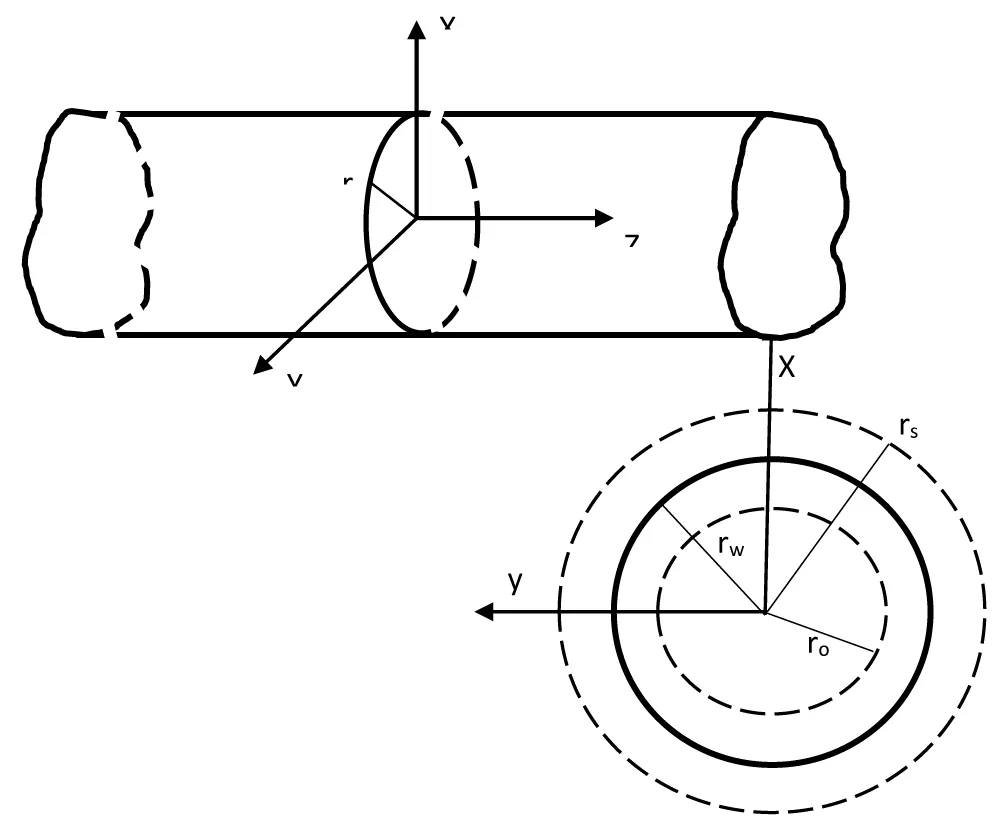
Let us consider the case when the plasma is placed in a cylindrical tube with a radius, and the waves propagate along the z - axis of the cylinder ( see Fig. 1).
According to Eq. (33), the cylindrical dependence of the spatial multiplier
on the coordinate , at the initial moment, can be represented in the form
. For later time, according to (C.1) (see Appendix C), we have
, (41)
where
and
are defined according to (C.2). Remembering the presence of a weak electric field, the expression (41) can be simplified (keeping the expression for the electric field only to the first power),
Fig. 1. Schematic view of a cylindrical tube and the main characteristic distances ( and radii ) in the cross section of a cylindrical pipe:
is the radius of the pipe, point
is the limit of the homogeneous region of the spatial multiplier, point
is located outside of the pipe and at this point the profile of the spatial multiplier becomes zero (see also Fig.2).
Figure 1: Schematic view of a cylindrical tube and the main characteristic distances ( and radii ) in the cross section of a cylindrical pipe: rw is the radius of the pipe, point r0 is the limit of the homogeneous region of the spatial multiplier, point rs is located outside of the pipe and at this point the profile of the spatial multiplier becomes zero (see also Figure 2).
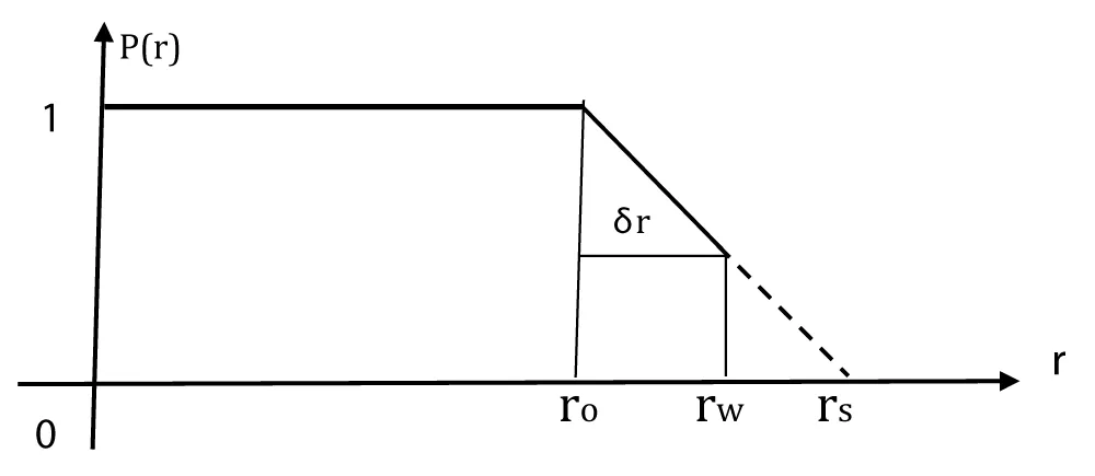
Figure 2: Dependence P(r) on the radial coordinate (r).
where the vector has only two radial components, and we have neglected terms of the order
. In the presence of a multiplier
(see Eq. (43)) and with a considerable value of the cylinder radius, the value (
) can be considered small. The cylinder, confining the plasma, can be described by the relation
, (43) where the general definition of the Heaviside step function is given by the relation
In fact, the multiplier (43) defines the radial shape of plasma characteristics. The wall of the cylinder is located at a distance from the axis of the cylinder. Here we will not discuss the structure of the layer adjoining the wall. Considering the thickness of this layer to be small, the profile of the special factor for the wall layer we have chosen in the form,
describing the linear reduction of the area under consideration to the bounded wall; rs is an auxiliary point for describing this descending area (rs is outside of the pipe).
Fig. 2. Dependence
on the radial coordinate
.
Plasma waves inside a cylindrical tube
We will start with the equation commonly used to treat longitudinal waves,
. Substituting expressions (39) and (42) into Eq. (46), we obtain
. Here we replaced integration over with the integration over
. Considering that in unperturbed plasma (in a plasma without an electric field) quasi-neutrality is preserved,
after multiplying terms in curly brackets of (47), the first term drops out according to (48). Taking into account the electric field only to the first power, from (47) we obtain
. (49) Substituting expressions (40) and (C.2) into (47) after integration over , we obtain:
where and
. In Eq. (50), we have used the relation
and the following integrations are performed:
The right-hand side of Eq. (53) for longitudinal waves gives
3.
The second derivative of expression (50) with time is equal to
Recalling the definition (3) of the value
and using (54), for the electric field we obtain :
or, after a simple transformation of the right-hand side:
Below we will look at plasma waves in a cylindrical pipe.
Waves inside the pipe
In this case, we assume that the waves propagate in the vicinity of the cylinder axis in the direction of the z-axis. According to the expressions (43), the spatial value
at
is equal to 1, and
at
is equal to zero, as
(see Eq. (43)). Neglecting terms with ion temperature, Eq. (56) becomes simplified and we obtain:
. (57) For waves propagating along the z-axis, are described by the equation:
. (58 For the frequency from Eq. (57) we have [3,4]:
Waves on the boundary wall
We can represent Eq. (56) in the form:
. After simply transforming the right-hand side of Eq. (60) and using the relation for cylindrical symmetry,
(of course, the second term on the right-hand side of Eq. (61) drops out due to cylindrical symmetry), we find
In the cylindrical model under consideration, we can assume that the radial component of the field is equal to zero inside the cylinder, as the radial gradient is absent. Due to the presence of broken places, the selected profile (43), shown in Fig.2, rather roughly describes the properties of plasma confinement. To bypass broken places in the boundaries of integration, we will replace with
, where
(and this replacement will be implied further). We integrate the near-wall region over a thin layer
, with a thickness
(
), assuming
. In the cylindrical variables, this integration takes the form:
Expanding the integrals (63) in a series in terms of degree
and taking into account the relation,
following from the definition (44), in the first approximation we obtain,
Collecting all the terms on the left-hand side of the equation and introducing the electron density as above,
, (66) we obtain the equation,
which describes the longitudinal wave,
, propagating along the boundary of the cylinder with a frequency:
Thus the character (dependences on time and coordinates) and frequency of waves propagating near the wall along the axis of a cylindrical pipe do not change (see also Eqs. (57)-(59)).
Summary
The analytic solution of the time-dependent Vlasov-Boltzmann kinetic equation, found in the present paper, in addition to time, also depends on spatial coordinates and velocity, which are solutions of characteristic equations for coordinates and velocity. In publications, in overwhelming cases, the dependence of the distribution function (DF) on velocity is discussed and used. In this paper, probably for the first time, an attempt is made to describe the coordinate dependence of the DF, obtained directly from the kinetic equation.
We consider plasma placed in a cylindrical confining tube. To simplify the problem, we consider the case when the plasma characteristics drop sharply in the radial direction at the boundary. Wave propagation near the cylinder axis and close to the surface of the tube is described.
Consideration of the case when plasma characteristics smoothly diminish to boundary values and analysis of the interaction of plasma particles with the wall require more careful and detailed consideration.
Appendix A
We start from the expression (16);
By renaming the variables
, .... and so on, we obtain expression (18),
Appendix B
Let’s start with Eq. (34) written in a form more convenient for analysis
Using expression (14) for the square of the value,
we find
Keeping the electric field strength only to the first power, and using the definition (10), from (B.2) we obtain
Now we can insert Eq.(B.3) into the expression (38), and after expanding the exponential function, we get Eqs. (39) and (40).
Appendix C
To simplify the expression for the spatial multiplier, we can repeat step by step the calculations performed in Appendix B. Using expressions (33) and (19), according to definitions (14) and (19), we obtain:
Let us again limit ourselves to taking into account the electric field to the first power. By introducing derivatives of expression (10) into Eq. (C.1), we obtain the equation:
The above expression (C.2) can be substituted into the equation (43). It is clear that terms containing to an odd power, as a result of integration over, give zero.



 Save to Mendeley