On Analytical Approximation of Cell Volume Distribution in Three-Dimensional Poisson-Voronoi Tessellation

Simulation of the cell volume distribution in the spatial Poisson-Voronoi tessellation

The dimensionless variables p and w for distance and cell volume (Eq. (1)) were used in the simulation. In a given series of computer experiments, the spatial Poisson-Voronoi tessellation was simulated in specimens that were cubes with a fixed edge L. We used the values of L from 20 to 40 in different series of computer experiments. The mean number density of nuclei in the dimensionless variables is equal to unity, and hence, the mean number of nuclei in a specimen was $L^3=8000-64000$ .

To determine the number $N_{c,j}$  of nuclei in each specimen j belonging to the series, a generator of pseudo-random numbers with a Poisson distribution and the mean value L3 was used. The random positions of nuclei, $x_{ji},y_{ji},z_{ji} (i=1,2,\dots ,N_{c,j})$  in specimen j were given by the pseudo-random number generator with uniform distribution over the interval .

Volumes of cells were calculated by numerical integration. To eliminate the surface effects in the calculation of the cell volume distribution, cells with nuclei located in a surface layer with the thickness ${\rho }_{sl}=1.8$  were ignored in the calculation of the mean volume and volume distribution. Several interior cells in a specimen j were denoted as $N_{ic,j}$ .

The probability density of the cell volume distribution was estimated using the calculated values of cell volumes and the kernel method with the Gaussian kernel [15] (see also Eq. (32) in Ref. [5]). The kernel method was used to determine a typical statistical error of the estimated probability density (see Sections 3.1.2, 3.3.1 and 3.3.2 in Ref. [15] and Eqs. (33)-(40) in Ref. [5]).

The simulation is described in detail in Ref. [5]. Note that the ensemble of cells used in the present paper for the Gaussian kernel estimation of the probability density of the cell volume distribution is more representative than that in Ref. [5].

Results of the simulation

Here we present the results of the simulation for cubic specimens with edge L = 40. The number of specimens in the series of computer experiments was J = 8500. As in Ref. [5], the sample of interior cells in the series was used for estimation of the average ${\omega }_a$ , the variance $\text{Var}\left(\omega ,\right)$  and the mean value $\langle {\omega }^3\rangle$ :

$\begin{array}{l}{N}_{ic}\cong 4.099\times {10}^8, {\omega }_a=1.00002\pm 0.00005, Var\left(\omega \right)\text{ (6)}\\ \cong 0.17905, {\omega }^3\cong 1.5967\pm 0.0003, \end{array}$

where N_ic is the number of interior cells in the series under consideration, and the statistical errors are given for the confidence level (the confidence coefficient) 0.99. To our knowledge, this is the largest data set for estimation of the cell volume distribution in the spatial Poisson-Voronoi tessellation. Data sets of  2.5 x 10⁸ and 3.6 x 10⁸  cells were used for this purpose in Refs. [3] (see Section IV.A) and [5] respectively.

This sample of interior cells was used for calculating the Gaussian-kernel estimator $f_{c,h}\left(\omega \right)$  of the probability density $f_c(\omega )$  of the cell volume distribution in the spatial Poisson-Voronoi tessellation. The calculation was carried out for discrete values of ${\omega }_i=0.02i (i=1, 2, \dots , 170)$  in the interval $0.02\le {\omega }_i\le 3.4$ . For the calculation of the kernel estimator $f_{c,h}\left({\omega }_i\right)$ , the optimal window width (smoothing parameter) was used

$: h_{opt}\cong 0.3686 N_{ic}^{-1/5}\cong 0.00698\cong 0.007,\text{ (7)}$

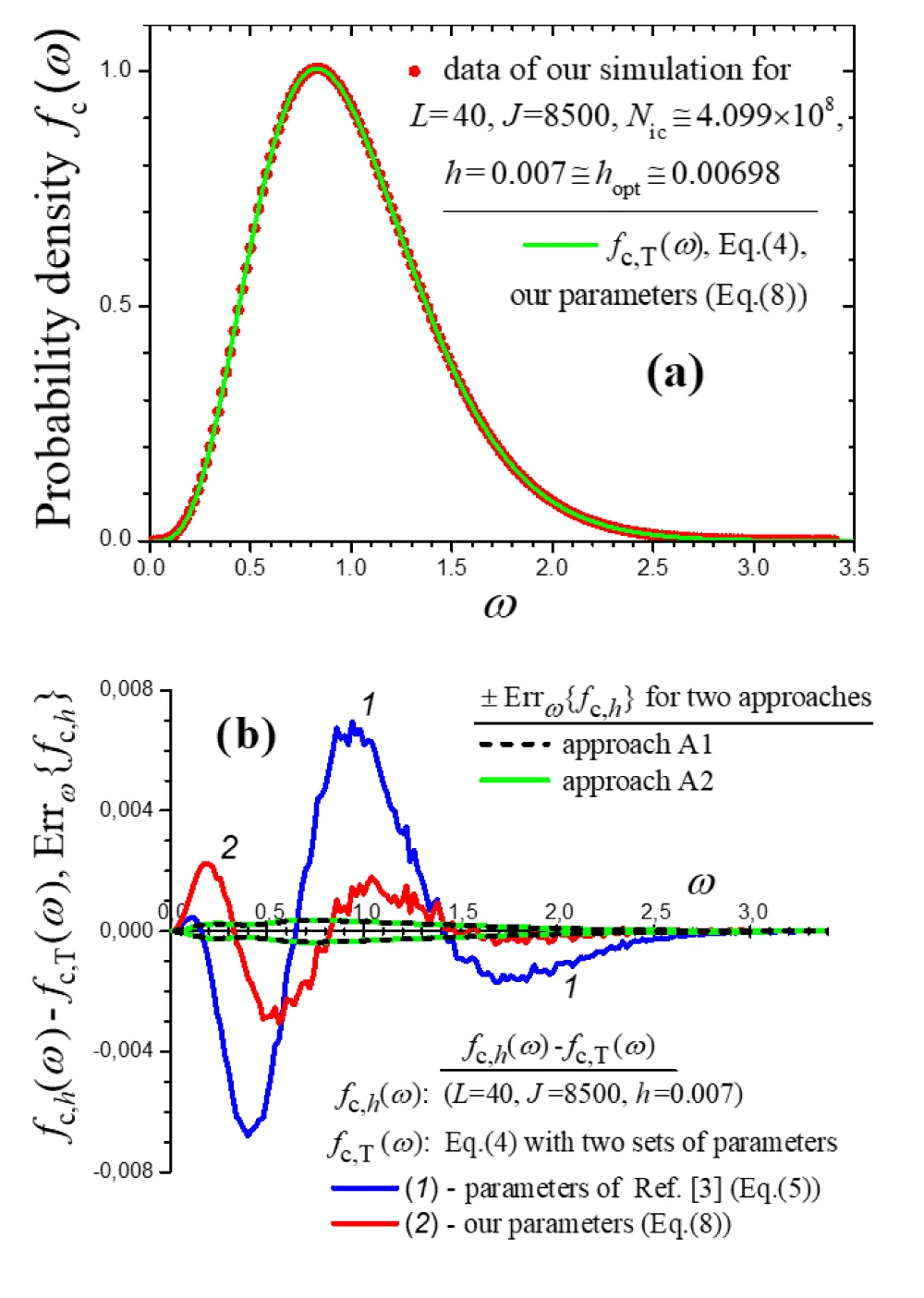
(see Eq. (39) of Ref. [5]) where the value of  N_ic is given in Eq. (6). The calculated values $f_{c,h}\left({\omega }_i\right)$  are presented in Figure 1a by circles.

The typical statistical errors $Er{r}_{\omega }\left\{f_{c,h}\right\}$  of the estimator $f_{c,h}\left(\omega \right)$  were calculated using two approaches A1 and A2 (see Eqs. (33)-(40) in Ref. [5]). The results of the calculation are shown in Figure 1b by black dotted and green solid curves for approaches A1 and A2, respectively. One can see that both approaches give typical error values which are approximately equal to each other. Maximum absolute values of the typical statistical error are less than  4 x 10^-4 and take place at $\omega \cong 0.7-0.8$ . As we concluded earlier ([5], p. 9, the end of the left column), the approaches A1 and A2 give a good description of the typical statistical error of the estimator $f_{c,h}\left(\omega \right)$ .

Figure 1: (a) The kernel estimator $f_{c,h}\left(\omega \right)$ of the probability density $f_c\left(\omega \right)$ of the cell volume distribution in the spatial Poisson-Voronoi tessellation obtained in our simulation and the approximate analytical probability density $f_{c, T}\left(\omega \right)$ (Eq. (4)) calculated with our set of parameters (Eq. (9)). (b) The difference between the kernel estimator $f_{c,h}\left(\omega \right)$ obtained in our simulation and the approximate analytical probability density $f_{c, T}\left(\omega \right)$ (Eq. (4)) calculated with two sets of parameters (Eq. (5) (curve 1) and Eq. (9) (curve 2)) in comparison with the typical statistical error of simulation $Er{r}_{\omega }\left\{f_{c,h}\right\}$ calculated using two approaches.

Comparison of the results of our simulation with those presented by Lazar et al. (2013)

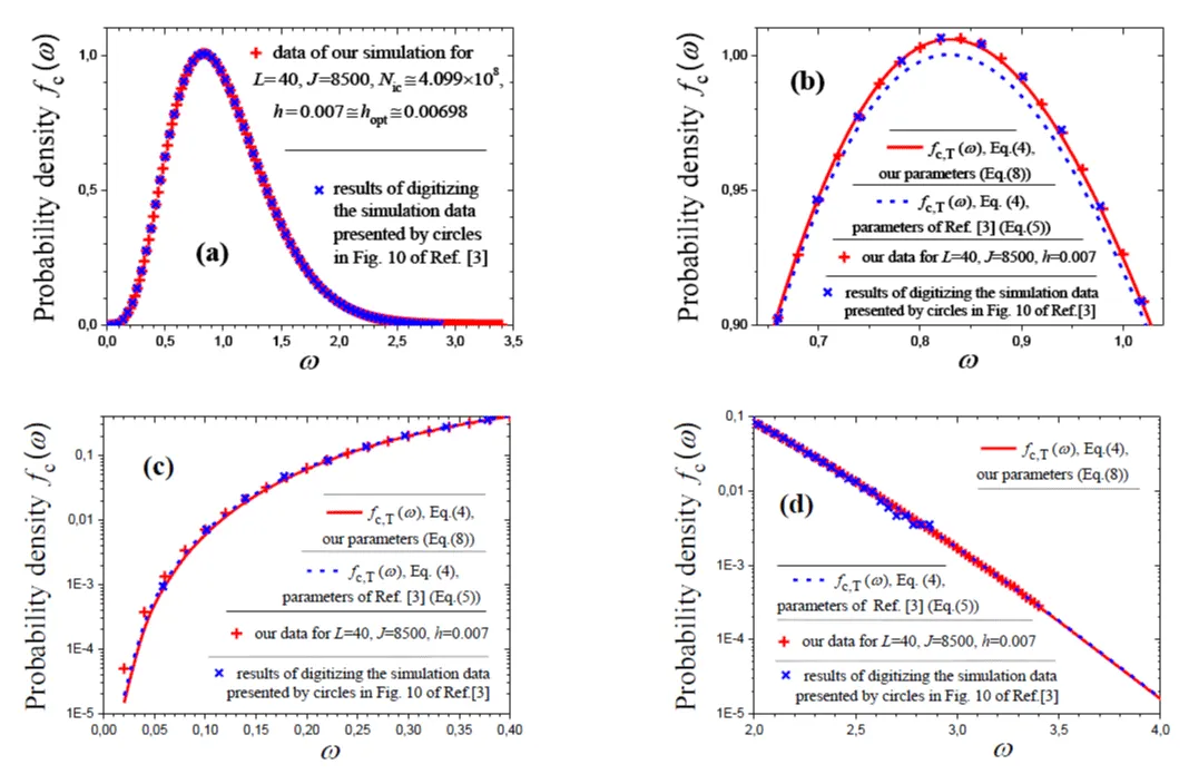
The graphical data on the probability density $f_c(\omega )$ of the cell volume distribution in the spatial Poisson-Voronoi tessellation are presented by circles in Fig. 10 of Ref. [3]. We digitized these data and compared the results of digitization with the estimator $f_{c,h}\left(\omega \right)$  presented in the previous section (Figure 2a-2d). Both sets of simulated values are found to be in good agreement. Some differences in the values (especially at $\omega =0.05$  and $\omega >2.6$ – see Figs. 2c and 2d, respectively) are obviously caused by errors of digitizing for small values of $f_c(\omega )$ .

Figure 2: The kernel estimator $f_{c,h}\left(\omega \right)$ of the probability density $f_c\left(\omega \right)$ of the cell volume distribution in the spatial Poisson-Voronoi tessellation obtained in our simulation and the results of digitizing the simulated probability density presented by circles in Fig. 10 of Ref. [3] in a wide interval of $\omega$ values (a), in the vicinity of the maximum (b) and in the ranges of small (c) and large (d) values of $\omega$ . The approximate analytical probability densities $f_{c, T}\left(\omega \right)$ (Eq. (4)) for two sets of parameters (Eqs. (5) and (9)) are also shown in parts (b)-(d).

We can also compare the values of the variance of cell volume distributions. The standard deviation ${\sigma }_{\omega }\cong 0.4231$ is given in the caption to Fig. 10 of Ref. [3]. This value corresponds to the variance $Var\left(\omega \right)={\sigma }_{\omega }^2\cong 0.17901,$  which is slightly less than the theoretical value $Var\left(\omega \right)\cong 0.17903$  given by Eq. (3). On the other hand, our value of variance, $\text{Var}\left(\omega \right)\cong 0.17905$ (Eq. (6)), is slightly greater than the theoretical one.

In addition, the positions of the maximum and the maximum values of the probability density are found to be the same in both simulations (see Ref. [5], p. 9, the end of the left column).

Thus, the results of the simulation carried out in Ref. [3] and our simulation are in good agreement.

Approximation of the probability density of the cell volume distribution in the spatial Poisson-Voronoi tessellation by the analytical function

As noted by Lazar et al. [3] and cited in Section 1, the three-parameter expression suggested by Tanemura (Eq. (4)) with the parameter values found in Ref. [3] (Eq. (5)) provides a best fit to the data simulated by these authors. To obtain these values of parameters, the authors used the exact values for the mean and variance (see Eqs. (2) and (3)), and a least-squares fit to the simulated data set.

However, Figure 10 of Lazar et al. [3] shows that in the vicinity of the maximum, the values of $f_{c, T}\left(\omega \right)$  (Eq. (4)) with parameter values found by these authors (Eq. (5)) are somewhat less than the simulated probability density. The same conclusion follows from Figure 2b, which gives a more detailed description of the probability density in the vicinity of the maximum.

To find a better analytical approximation of the simulated probability density by expression $f_{c, T}\left(\omega \right)$ (Eq. (4)), we used for determination of parameter values a method somewhat different from that used in Ref. [3]. We imposed three conditions on parameters $\alpha , \beta$  and γ:

$\omega =\underset{0}{\overset{\infty }{{\displaystyle \int }}}\omega f_{c,T}\left(\omega \right)d\omega =\frac{\Gamma \left[\left(\gamma +1\right)/\alpha \right]}{{\beta }^{1/\alpha }\Gamma (\gamma /\alpha )}=1 , \text{ (8a)}$

${\omega }^2=\underset{0}{\overset{\infty }{{\displaystyle \int }}}{\omega }^2{f}_{c,T}\left(\omega \right)d\omega =\frac{\Gamma \left[\left(\gamma +2\right)/\alpha \right]}{{\beta }^{2/\alpha }\Gamma (\gamma /\alpha )}=1+Var(\omega )\cong 1.1790324 , \text{ (8b)}$

${\omega }^3=\underset{0}{\overset{\infty }{{\displaystyle \int }}}{\omega }^3{f}_{c,T}\left(\omega \right)d\omega =\frac{\Gamma \left[\left(\gamma +3\right)/\alpha \right]}{{\beta }^{3/\alpha }\Gamma (\gamma /\alpha )}\cong 1.5967\text{ (8c)}$

(Note that $f_{c, T}\left(\omega \right)$  is normalized for any values of parameters). The first two conditions (Eqs. (8a) and (8b)) are the same as those used in Ref. [3]. The value of $\langle \omega \rangle =1$  is connected with the choice of the dimensionless distances (Eqs. (1) and (2)). For $Var(\omega ),$  we took the theoretical value (Eq. (3)). The value of $\langle {\omega }^3\rangle$  was determined in our computer experiments (Eq. (6)). These three conditions (Eqs. (8a), (8b), and (8c)) were considered as a system of three equations for parameters $\alpha , \beta and\gamma$ . We solved the system numerically using various guess values for parameters (including values determined in Ref. [3] (see Eq. (5)) or by Tanemura [14], or even the simplest ones, $\alpha =\beta =\gamma =1$ ) and obtained the same solution:

$\alpha \cong 1.14373, \beta \cong 4.21631, \gamma \cong \mathrm{4.89155.} \text{ (9)}$

It should be noted that these values of parameters ensure the fulfillment of Eqs. (8a), (8b) and (8c) with an accuracy of,  $\cong 2\times {10}^{-6}, \cong 6\times {10}^{-6}$ , and $\cong {10}^{-5}$ , respectively (Table 1). The values

$\alpha \cong 1.14373229793, \beta \cong 4.21630858859, \gamma \cong 4.89154717005\text{ (10)}$

lead to the practically exact fulfilment of Eqs. (8a)-(8c) (Table 1). However, we showed that the accuracy of the representation of the parameters used in Eq. (9) is quite sufficient for the calculation of the function $f_{c, T}\left(\omega \right)$ (Eq. (4)).

We used three mean values, $\langle \omega \rangle ,\langle {\omega }^2\rangle and\langle {\omega }^3\rangle ,$  to determine the approximation parameters in Eq. (4). These mean values are simple analytical functions of the approximation parameters, and the system of three equations is easily solved numerically and has the same solution for a variety of guess values for parameters. The resulting approximation describes the simulation results well (Table 1). The proposed method is simple to implement compared to the least-squares method, which can also lead to unsatisfactory approximation (see Section 6).

It should also be noted that, if desired, one can use a similar method with another parameter instead of $\langle {\omega }^3\rangle ,$  such as the mode or higher-order moment. However, this parameter must be known from computer simulation or from theoretical considerations.

The function $f_{c, T}\left(\omega \right)$  with parameters given in Eq. (9) provide a much better description of the simulated probability density in the vicinity of the maximum than the function $f_{c, T}\left(\omega \right)$  with parameter values found in Ref. [3] and reproduced by Eq. (5) (Figure. 2b). The two descriptions give close results in the range of small values of  (Figure 2c) and do not differ appreciably in the range of large values of  (Figure 2d).

It should also be noted that the simulated probability density $f_c(\omega )$  is presented in Ref. [3] (the inset in Fig. 10) up to a value of $\omega \cong 5,$  which is significantly greater than the maximum volume value in our simulation ( $\omega =3.4$ ). In the whole range of large values of volume, $2<\omega <5$ , the probability density simulated in Lazar et al. (2013) is well described by the analytical function $f_{c, T}\left(\omega \right)$ (Eq. (4)) with parameters proposed by these authors (see Eq. (5)). Because the analytical functions $f_{c, T}\left(\omega \right)$  for both sets of parameters (Eqs. (5) and (9)) are close to each other in the range $2<\omega <5$ (Figure. 2d, dots and solid line), we can conclude that the function $f_{c, T}\left(\omega \right)$  with our set of parameters (Eq. (9)) gives a good description of simulation data at least up to $\omega =5$ .

Figure 1b shows the difference between the simulated probability density $f_{c, T}\left(\omega \right)$  ( $L=40, J=8500, h=0.007\cong h_{opt}\cong 0.00698$ ) and the analytical function $f_{c, T}\left(\omega \right)$  calculated with two sets of parameters (Eqs. (5) and (9)):

$\begin{array}{l}{r}_i=f_{c,h}\left({\omega }_i\right)-f_{c,T}\left({\omega }_i\right), i=1,2,\dots ,170, \text{ (11)}\\ {\omega }_i=0.02 i, A={\displaystyle \sum }_{i=1}^{170}\left|r_i\right|, S={\displaystyle \sum }_{i=1}^{170}{r}_i^2.\end{array}$

The difference presents an error (residual) ri of the approximation of the simulation results by the analytical function. The total difference is characterized by the values of A and S, the latter being used in the least squares method. The residual curves (Figure 1b, curves 1 and 2) demonstrate irregular fine structure (the ripple structure) caused by the statistical nature of $f_{c,h}\left(\omega \right)$ , and the “amplitude” of the ripple structure is approximately equal to the typical statistical error of simulation $Er{r}_{\omega }\left\{f_{c,h}\right\}$  shown in the same figure. The residuals calculated for other series of computer experiments differ from those presented in Figure 1b only in the ripple structure, while the general form of the curves remains practically unchanged.

Residuals curves (curves 1 and 2 in Figure 1b,) show that our set of parameters (Eq. (9)) gives a significantly better approximation of the simulation results in comparison with the set proposed in Ref. [3] (Eq. (5)). The conclusion is confirmed by estimation of the sum of absolute values of residuals, A, and of the sum of squared residuals, S (Eq. (11)). The results of the estimation are presented in Table 1 and show that we reduced A and S by a factors of 3.0 and 7.8, respectively. In particular, our parameters are preferable from the point of view of the least squares method, since they lead to a smaller value of S.

Discussion

According to the analysis presented above (Section 4 and Figure 2), one can conclude that our numerical simulation of the cell volume distribution leads to results that are in good agreement with the results of the most representative previous simulation carried out in Ref. [3].

It should be noted that Lazar et al. [3] do not specify how the values of the simulated volume distribution density presented in Fig. 10 of their paper were calculated and do not give the errors of these calculations. It may be assumed that in these calculations the density was calculated as a histogram.

For the calculation of the probability density of the cell volume distribution in the spatial Poisson-Voronoi tessellation, we used the kernel method with the Gaussian kernel. This method allows one not only to calculate the probability density $f_{c,h}\left(\omega \right)$  (Figure 1a) but also to estimate its typical statistical error $Er{r}_{\omega }\left\{f_{c,h}\right\}$ (Figure 1b).

Although the probability densities simulated in Ref. [3] and in the present paper are in good agreement (Figure 2), the accuracy of their analytical approximation by Eq. (4) is significantly better if our parameters (Eq. (9)) are used instead of the parameters (Eq. (5)) proposed in Ref. [3] (Figure 2b).

In our opinion, insufficient accuracy of the approximation given in Lazar et al. (2013) may be caused by a manifestation of a local minimum in the least-squares fit to the simulated data set carried out in this reference. Indeed, in the case of non-linear least squares approximation with several parameters, the sum  of squares of approximation errors (residuals) (Eq. (11)) as a function of parameters “may be very complicated, in particular, it may possess numerous local extrema” (Riley et al., 2006). Frequently, the procedure of minimizing will converge to the local minimum ‘nearest’ to the initial values of parameters (the first guess). Using another starting point in $\alpha -\beta -\gamma$ space, one can find another minimum which may be less or greater than the previous one. Since, in fact, we are interested only in the local minimum that has the absolute lowest value of the sum S, it is clear that a large part of solving the problem is to make a ‘good’ first guess. In our method of determination of the parameters (solving the system of Eqs. (8a)-(8c)), difficulties of a ‘good’ first guess are avoided.

Let us compare the analytical approximations discussed above with three other approximations proposed earlier. To approximate the simulated probability density, Kiang [9] proposed the γ-distribution

$f_{c,K}\left(\omega \right)\cong p{\left(p\omega \right)}^{p-1}\text{ exp}(-p\omega )/\Gamma \left(p\right),\text{ (12)}$

which is normalized to unity and gives the average volume ${\omega }_a=1$  and the variance $Var\left(\omega \right)=1/p$ . This distribution with values of p from $\cong 5.3to\cong 6.2$ was used by many authors for analytical approximation of simulated data on the volume distribution of the 3D Poisson-Voronoi tessellation (see, for example, [3,5,9-11,13,17-19]). In particular, it was shown [17] that the γ-distribution with the parameter value of $p=5.586$ , which gives the variance $Var\left\{\omega \right\}=1/p\cong 0.179$  close to the theoretical one (Eq. (3)), provides a good fit to simulated data. Figure 3 shows the γ-distribution $f_{c, K}\left(\omega \right)$  with the parameter value of $p=5.58558$ , which gives the variance $\text{Var}\left\{\omega \right\}=1/p\cong 0.1790324371$  equal to the theoretical one with the absolute accuracy of $1\times {10}^{-9}$ . For comparison, the simulated probability density $f_{c,h}\left(\omega \right)$ (the same as in Figures 1a and 2) and the analytical probability densities $f_{c, T}\left(\omega \right)$ (Eq. (4)) for two sets of parameters (Eqs. (5) and (9)) are also shown in Figures 3a-3c.

Figure 3: (a-c): Different analytical approximations of the probability density $f_c\left(\omega \right)$  of the cell volume distribution in the spatial Poisson-Voronoi tessellation in comparison with the kernel estimator $f_{c,h}\left(\omega \right)$  obtained in our simulation in the vicinity of the maximum (a), and in the ranges of small (b) and large (c) values of the dimensionless cell volume . (d): The difference between the kernel estimator $f_{c,h}\left(\omega \right)$  and the approximate analytical probability density $f_{c, T}\left(\omega \right)$ (Eq. (4)) calculated with four sets of parameters presented in Ref. [3] (Eq. (5), curve 1), Ref. [14] (Eq. (14), curve 3) and this work (Eq. (9), curve 2 and Eq. (15), curve 4).

One can see (Figure 3a-3c) that the approximation by the one-parameter g-distribution (Eq. (12)) with the parameter value of $p=5.58558$  is inaccurate in the vicinity of the maximum, and in the ranges of small and large values of the dimensionless cell volume $\omega$

The three-parameter g-distribution (Eq. (4)) with the parameters proposed in Lazar et al. (2013) cannot ensure a good approximation of the simulated data in the vicinity of the maximum (Figure 3a). Our set of parameters (Eq. (9)) gives a much better approximation as illustrated by Figure 3d. As noted in the end of the previous section, this conclusion is confirmed by values of A and S presented in Table 1.

It is interesting to present the function $f_{c, T}\left(\omega \right)$ (Eq. (4)) with two sets of parameters found by Tanemura [12,14]. The first set is cited by Lazar et al. [3] as a result of Tanemura [14]:.

$\alpha =1.409, \beta =2.813, \gamma =\mathrm{4.120.}\text{ (13)}$

However, this citation is incorrect. Indeed, this set is mentioned in Section 5 (p. 247) of Tanemura's paper [14] with reference to an earlier work [12] of Tanemura, where these values of the parameters were obtained on the basis of the results of computer simulation.

Lazar et al. [3] also stated that the generalized gamma distribution (Eq. (4)) was suggested by Tanemura [14], whereas the references presented in papers [12,20] show that it was proposed much earlier [21] for approximation of the cell area distribution in the 2D Poisson-Voronoi tessellation. The first application to the 3D case was presented in paper [12] by Tanemura.

Tanemura [14] used a larger simulated data set for the 3D case (5 x 10⁵ cells) than earlier [12] (105 cells) and obtained the following values of parameters (see Table 9(a) on page 244 of Ref. [14])

$\alpha =1.16788, \beta =4.04039, \gamma =4.79803\text{ (14)}$

for analytical approximation of the simulated histogram by the generalized gamma distribution (Eq. (4)) (see Figure 8 in Ref. [14]). This set of parameters is not mentioned by Lazar et al. [13].

The generalized gamma distributions $f_{c, T}\left(\omega \right)$  (Eq. (4)) with these two sets of parameters (Eqs. (13) and (14)) are also shown in Figure 3. One can see that the approximation by the function $f_{c, T}\left(\omega \right)$  with parameters proposed by Tanemura in Ref. [12] (Eq. (13)) is not very good, and its accuracy is comparable with the accuracy of approximation by the one-parameter γ-distribution $f_{c, K}\left(\omega \right)$ (Eq. (12)) with the parameter value of $p=5.58558$ . Figure 3a shows that parameters proposed by Tanemura later [14] (Eq. (14)) lead to significantly better description of our simulation data in the vicinity of the maximum than the parameters of Lazar et al. [3] (Eq. (5)). The differences between the simulated and analytical probability densities (Figure 3d) indicate that the approximations by the functions $f_{c, T}\left(\omega \right)$  with the Tanemura parameters (Eq. (14)) and our parameters (Eq. (9)) give close accuracies, while the approximation with parameters of Lazar et al. [3]) (Eq. (5)) is much less accurate.

To confirm this conclusion quantitatively, we evaluated the sum of absolute values of residuals, A, and the sum of squared residuals, S, (Eq. (11)), for the case of the Tanemura parameters [14] (Eq. (14)) (Table 1). Comparison of the data presented in Table 1 shows that the Tanemura approximation [14] is significantly better than that of Lazar et al. [3], and is somewhat better than our approximation with respect to the value of the sum of squared residuals, S.

In addition, we approximated the simulated probability density $f_{c,h}\left(\omega \right)$  ( $L=40, J=8500, h=0.007\cong h_{opt}\cong 0.00698$ ) by the analytical function $f_{c, T}\left(\omega \right)$  using the least squares method. We were looking for an unconstrained minimum of a squared residuals sum, S, as a function of parameters $\alpha , \beta ,and\gamma$ . (It should be noted that in Ref. [3] two conditions (Eq. (8a) and (8b)) were imposed on the parameters, and only one free parameter was considered). As a result, we obtained the following values

$\alpha =1.16239, \beta =4.09048, \gamma =4.83211, \text{ (15)}$

which leads to the least value of  among the values given in Table 1. For this set of parameters, the value of A is also appreciably less than for other approximations in Table 1. Figure 3d also shows that the difference between the simulated kernel estimator $f_{c,h}\left(\omega \right)$  and this analytical approximation is less than for other approximations discussed in the present paper. Hence, this analytical approximation gives the best description of the results of our modeling of the distribution of cell volumes in the spatial Poisson-Voronoi tessellation.

On the other hand, there is another criterion for the applicability of the approximation: accuracy of fulfilment of Eqs. (8a)-(8c) for the mean values $\langle \omega \rangle ,\langle {\omega }^2\rangle and\langle {\omega }^3\rangle$ , In this respect, the parameters given by Eq. (9) are good, and the parameters of Eq. (11) are ideal.

The choice of one (Eq. (15)) or another (Eq. (11)) set of parameters depends on the purpose of the approximation.

Conclusion

The cell volume distribution in the spatial Poisson-Voronoi tessellation is simulated using @ 4.099´10⁸ cells. Previously, the most representative simulation was carried out by Lazar et al., where 2.5´10⁸ cells were used.

To calculate the probability density of the cell volume distribution in the spatial Poisson-Voronoi tessellation, the kernel method with the Gaussian kernel is applied to the data set of cell volumes obtained in our simulation. The method provides a possibility of estimating the statistical error of probability density calculation. Maximum absolute values of the typical statistical error are less than 4´10^-4.

The probability densities obtained in our simulation and in the simulation of Lazar et al. are found to be in good agreement.

Analytical approximation of the probability density obtained in our simulation by the generalized gamma distribution with different sets of parameters is discussed. We show that the set of parameters proposed by Lazar et al. does not lead to a satisfactory analytical approximation not only of our simulation results, but also of the results of Lazar et al.

We note that citation of Tanemura by Lazar et al. is incorrect. The correct citation shows that the parameters proposed by Tanemura in 2003 lead to a significantly better description of our simulation data (and of the data obtained by Lazar et al.) than the parameters proposed by Lazar et al.

We propose a method for determining the parameters of the generalized gamma distribution that provides the required values of the mean volume, mean squared volume, and mean cubed volume of cells. The mean volume is equal to unity and is determined by the dimensionless formulation of the problem. The value of the mean squared volume was calculated theoretically by a number of authors. The value of the mean cubed volume may be taken from the simulation. As a result, we obtain a system of three equations for three parameters of the generalized gamma distribution. The solution of this system leads to the approximation whose accuracy is close to that of the Tanemura approximation.

Finally, we use the least squares method to obtain values of the three parameters for approximating the probability density obtained in our simulation by the generalized gamma distribution. This approach gives the best analytical approximation for the results of our modeling of the distribution of cell volumes in the spatial Poisson-Voronoi tessellation.

Data availability

The data that support the findings of this study will be made available from the author on request.