Implicit Function-based 3D Reconstruction for Point Cloud Data

Normal estimation of point clouds and normal orientation consistency

Normal estimation of point clouds based on covariance matrix

Normal estimation is a critical component of point cloud processing, playing a fundamental role in 3D reconstruction, surface fitting, feature extraction, and classification. Normal information describes the local geometric properties of point clouds and is essential for applications such as surface rendering, mesh reconstruction, and point cloud registration.

The covariance matrix-based method is a classical and efficient approach to normal estimation, relying on the statistical distribution of local neighborhoods. By applying Principal Component Analysis (PCA) to the covariance matrix, the normal direction is identified as the eigenvector associated with the smallest eigenvalue. Owing to its mathematical simplicity and computational efficiency, this method has been widely adopted in point cloud processing.

(1) Local Neighborhood Search: To estimate the normal at a point p_i, its local neighborhood N(p_i) must be identified. Common strategies for neighborhood selection include:

k-Nearest Neighbors (k-NN): Identifies the k closest points to p_i, based on Euclidean distance.

Fixed Radius Search: Selects all points within a given radius r centered at p_i.

Let the neighborhood of p_i contain n points, denoted as $N\mathrm{<mo\; stretchy="false">(</mo>}{p}_i\mathrm{<mo\; stretchy="false">)</mo><mo>=</mo><mo>\{</mo>}{p}_1\mathrm{,}{p}_2\mathrm{,...,}{p}_n\mathrm{<mo>\}</mo>}$ .

(2) Covariance Matrix Computation: In point cloud normal estimation, the covariance matrix is typically constructed with respect to a reference point. This reference can be either the current point under consideration or the centroid (mean) of its neighborhood, computed as :

$\overline{q}\mathrm{<mo>=</mo>}\frac{1}{n}{\displaystyle {\sum }_i^n{q}_i}\mathrm{<mo>=</mo>}\left(\frac{1}{n}{\displaystyle {\sum }_i^n{q}_{xi}}\mathrm{,}\frac{1}{n}{\displaystyle {\sum }_i^n{q}_{yi}},\frac{1}{n}{\displaystyle {\sum }_i^n{q}_{zi}}\right)\text{ (1)}$

The covariance matrix is then computed as:

$C\mathrm{<mo>=</mo>}\frac{1}{n}{\displaystyle {\sum }_i^n{q}_i}\mathrm{<mo>=</mo>}\left(q_i-\overline{q}\right){\left(q_i-\overline{q}\right)}^T\text{ (3)}$

Where p_i represents the coordinates of the neighboring points. The covariance matrix C is a 3 × 3 symmetric matrix:

$C\mathrm{<mo>=</mo>}\left[\begin{array}{ccc}{C}_{xx}& C_{xy}& C_{xz}\\ C_{yx}& C_{yy}& C_{yz}\\ C_{zx}& C_{zy}& C_{zz}\end{array}\right]\text{ (3)}$

Each element C_uv is calculated as:

$C_{uv}\mathrm{<mo>=</mo>}\frac{1}{n}{\displaystyle {\sum }_i^n\mathrm{<mo\; stretchy="false">(</mo>}{u}_i-\overline{u}\mathrm{<mo\; stretchy="false">)</mo><mo\; stretchy="false">(</mo>}{v}_i-\overline{v}\mathrm{<mo\; stretchy="false">)</mo>}}\text{ (4)}$

where u,v represents the x,y,z coordinates.

(3) Eigenvector computation: Perform Eigen Decomposition on the covariance matrix C, obtaining eigenvalues ${\lambda }_1\mathrm{,}{\lambda }_2\mathrm{,}{\lambda }_3$ and their corresponding eigenvectors v₁, v₂,v₃ , where:

${\lambda }_1\ge {\lambda }_2\ge {\lambda }_3\text{ (5)}$

The smallest eigenvalue l3 corresponds to the eigenvector v3, which represents the least variance direction in the local neighborhood. This vector is chosen as the estimated normal:

n_i = v₃ (6)

Normal orientation consistency

In point cloud normal estimation, particularly with covariance matrix-based methods, the computed normals inherently exhibit directional ambiguity, both ni and -ni are valid normal at a point pi . Without resolving this ambiguity, inconsistent normal directions can cause significant errors in surface reconstruction, rendering, or registration. Therefore, enforcing consistent normal orientation across the point cloud is essential.

This paper adopts a hybrid strategy that combines local consistency with neighborhood-based propagation. Specifically, a set of seed points is selected from the point cloud, these are typically representative points. The normal directions of these seed points serve as the initial references for propagation. From each seed point, normal directions are locally propagated to neighboring points based on a directional consistency criterion.

To ensure the initial consistency of normal orientations at the seed points, which serve as the starting nodes for orientation propagation, this paper adopts a method based on quadratic surface fitting to refine and correct their normal directions.

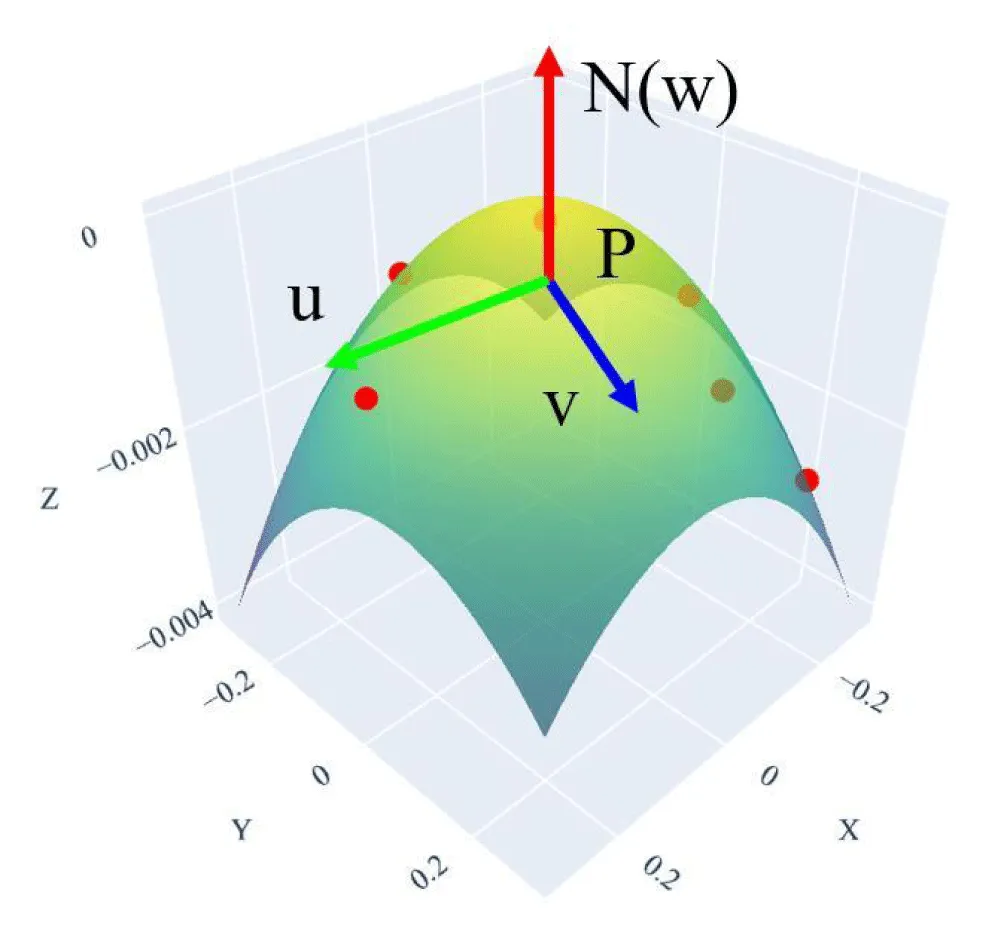
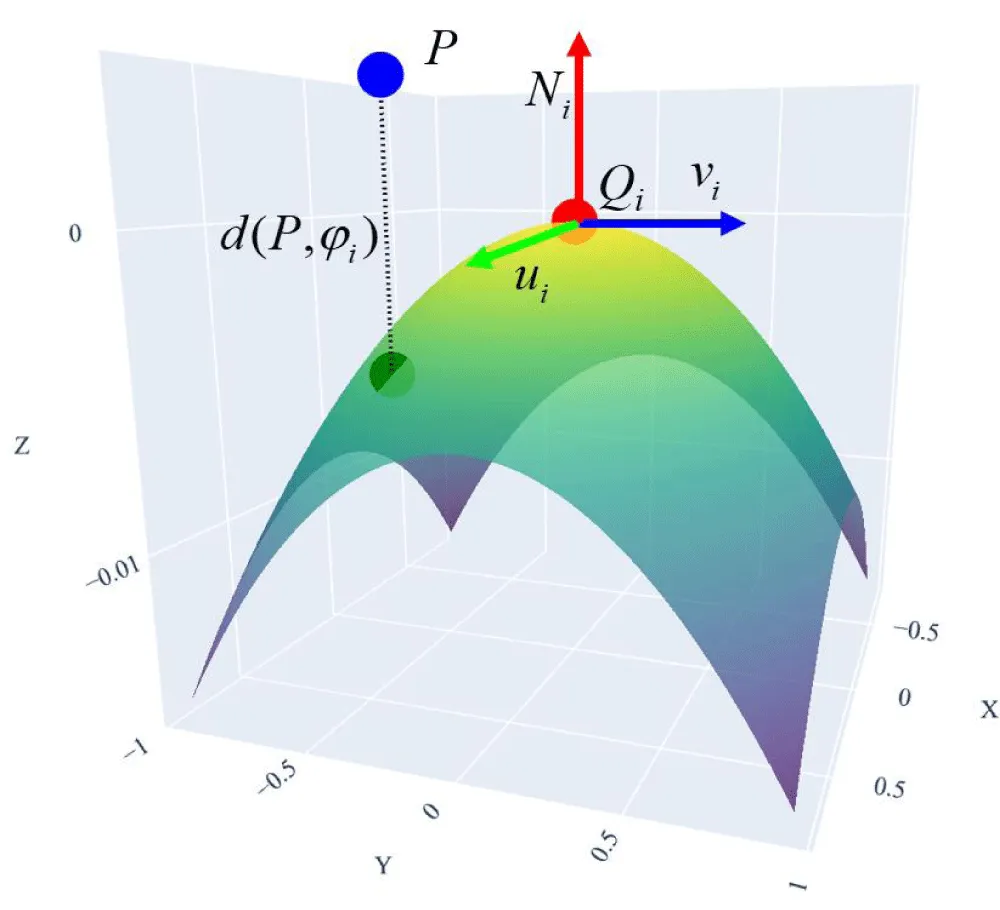
Local quadratic surface fitting method: To accurately capture the local geometric characteristics of a point cloud, we adopt a local coordinate-based quadratic surface fitting approach centered at a given point. This method involves establishing a local frame aligned with the surface normal and fitting a second-order surface to the nearest neighboring points in that frame, as shown in Figure 1. The procedure is detailed as follows:

Figure 1: Local Coordinate-Based Quadratic Surface Fitting.

1) Selection of Neighboring Points

Given a query point $P\in {ℝ}^{}$ with a corresponding unit surface normal vector $N\in {ℝ}^{}$ , we identify its k nearest neighbors from a global point set $Q\mathrm{<mo>=</mo>}{\left\{q_i\right\}}_{i\mathrm{<mo>=</mo>1}}^n\in {ℝ}^3$ , using Euclidean distance as the metric. In this paper, we set k = 6.

2) Construction of Local Coordinate System

A local right-handed orthonormal coordinate system (u,v,w) is established at P , where:

w = N defines the local z-axis direction;

u is obtained by normalizing the cross product of N with an arbitrary non-collinear vector t , $u\mathrm{<mo>=</mo>}\frac{t\times N}{\Vert t\times N\Vert }$ , v = u × w . The resulting rotation matrix $R\mathrm{<mo>=</mo>}{\left[u^{\text{T}}{v}^{\text{T}}{w}^{\text{T}}\right]}^{\text{T}}\in {ℝ}^{3\times 3}$ transforms global coordinates into the local frame. For each neighboring point q_j, the local coordinate $q_j^L$ is computed as:

$q_j^L\mathrm{<mo>=</mo>}R\mathrm{<mo\; stretchy="false">(</mo>}{q}_j-p\mathrm{<mo\; stretchy="false">)</mo>}\text{ (7)}$

3) Quadratic Surface Fitting in the Local Fram

After transformation, the neighboring points are represented in the local frame as $q_j^L\mathrm{<mo>=</mo><mo\; stretchy="false">(</mo>}{x}_j\mathrm{,}{y}_j\mathrm{,}{z}_j\mathrm{<mo\; stretchy="false">)</mo>}$ . We assume the local surface (as shown in Figure 1) near P can be approximated by a second-order polynomial of the form:

$z\mathrm{<mo>=</mo>}a{x}^2+2bxy+c{y}^2\text{ (8)}$

To estimate the coefficients a, b, c we construct a linear system using the transformed coordinates:

Z = AX (9)

where:

$Z\mathrm{<mo>=</mo>}\left(\begin{array}{c}{z}_1\\ z_2\\ ⋮\\ z_6\end{array}\right)\mathrm{,}A\mathrm{<mo>=</mo>}\left(\begin{array}{ccc}{x}_1^2& 2x_1{y}_1& y_1^2\\ x_2^2& 2x_2{y}_2& y_2^2\\ ⋮& ⋮& ⋮\\ x_6^2& 2x_6{y}_6& y_6^2\end{array}\right)\mathrm{,}X\mathrm{<mo>=</mo>}\left(\begin{array}{c}a\\ b\\ c\end{array}\right)\text{ (10)}$

The coefficients are then estimated via the least-squares solution:

$X\mathrm{<mo>=</mo><mo\; stretchy="false">(</mo>}{A}^{\text{T}}A{\mathrm{<mo\; stretchy="false">)</mo>}}^{-1}{A}^{\text{T}}Z\text{ (11)}$

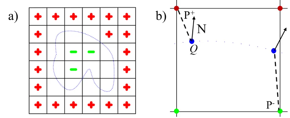
Normal consistency by local quadratic surface: To ensure the initial consistency of the normal orientations at the seed points, the entire point cloud is first enclosed within a uniform volumetric grid of resolution 50 × 50 × 50 . Each grid vertex is then classified as lying either outside or inside the surface: vertices outside are assigned a positive sign (“+”), while those inside are assigned with a negative sign (“–”), as shown in Figure 2a). This initial classification provides a coarse signed distance field used for orientation refinement in subsequent steps.

Figure 2: a) Inside and outside vertex classification in a volumetric grid. b) Closest point method for normal orientation.

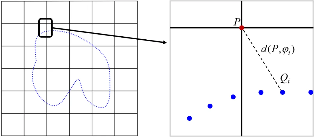
For each grid vertex P located near the surface boundary, the closest point Q on the input point cloud is identified, as illustrated in Figure 2b). A local coordinate system is constructed at Q, with the local z-axis is aligned to the normal vector N at that point. Within this local frame, the quadratic surface defined in Equation 8, is fitted to the neighboring points. This fitted surface serves as a smooth approximation of the local geometry near Q. Using the fitted coefficients a, b, c , the function is evaluated at the offset points P⁺ and P^-, which are positioned slightly along the positive and negative directions of the normal vector, respectively:

$\psi \mathrm{<mo\; stretchy="false">(</mo>}P\mathrm{<mo\; stretchy="false">)</mo><mo>=</mo>}a{x}_P^2+2b{x}_p{y}_P+c{y}_P^2\text{ (12)}$

If the evaluated function Ψ at either offset point yields a sign inconsistent with the expected orientation $\psi \mathrm{<mo\; stretchy="false">(</mo>}{P}^{+}\mathrm{<mo\; stretchy="false">)</mo><mo><</mo>0}$ or $\psi \mathrm{<mo\; stretchy="false">(</mo>}{P}^{-}\mathrm{<mo\; stretchy="false">)</mo><mo>></mo>0}$ , then the normal vector is flipped as N = -N , and the coefficients are adjusted accordingly $a\mathrm{<mo>=</mo>}-a\mathrm{,}b\mathrm{<mo>=</mo>}b\mathrm{,}c\mathrm{<mo>=</mo>}-c$ .

This correction ensures that the fitted surface's normal direction points consistently outward from the shape, resolving ambiguities in surface orientation near thin or concave regions. After obtaining a reliable and consistently oriented normal at the selected seed points using quadratic surface fitting, the method proceeds to propagate the corrected normal directions to the rest of the point cloud using a neighborhood-based orientation propagation algorithm.

In this process, each seed point acts as a local root, and its normal direction is propagated to neighboring points in a breadth-first manner. At each propagation step, if the dot product between the current point's normal and that of its neighbor is negative, the neighbor's normal is flipped to align with the propagation direction.

By employing multiple seed points and performing propagation in parallel across the dataset, this method ensures global orientation consistency while avoiding issues such as direction drift or error accumulation that may arise from using a single-root traversal.

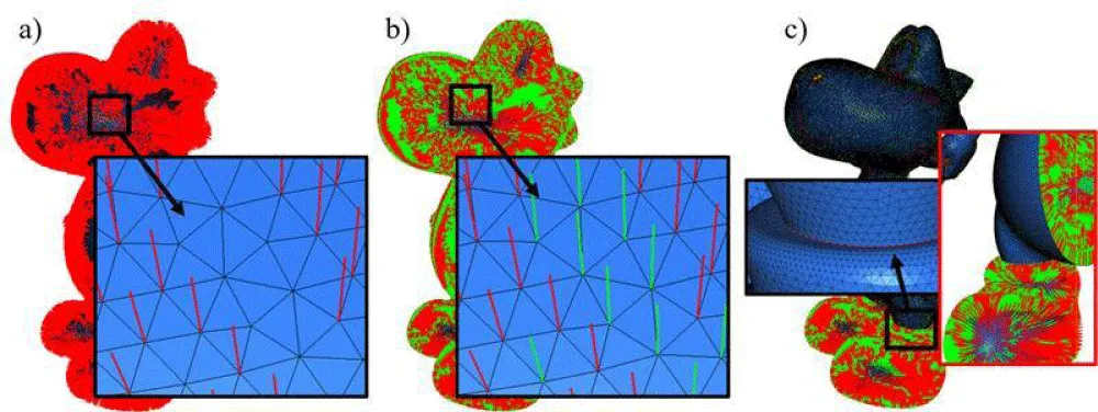
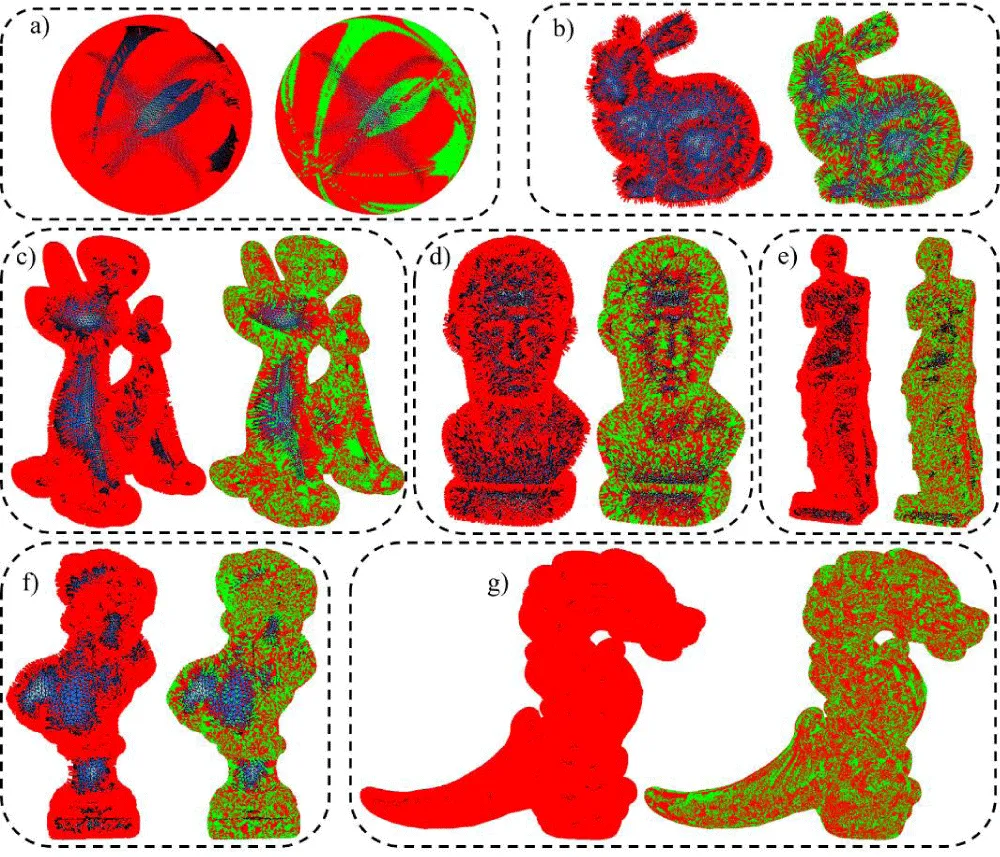
The results of the normal orientation correction are shown in Figure 3. As shown in Figure 3a), the initial normal vectors are inconsistent, with some pointing inward and others outward. After applying the proposed method, a globally consistent normal field is obtained. In Figure 3b), the red vectors represent the normal that were already correctly oriented, while the green vectors denote those that were originally inverted but have been successfully corrected to point outward. Figure 3c), shows the result obtained using a traditional method. It can be observed that in regions with complex geometric structures, such as corners and edges, the normal vectors remain noticeably disordered and lack global consistency. Specifically, the normals in the upper part of the model tend to point inward, while those in the lower part point outward, further highlighting the limitations of traditional methods in achieving globally consistent normal orientation. This demonstrates the effectiveness of the proposed strategy in producing coherent and meaningful normal directions across the entire point cloud.

Figure 3: Normal reorientation: a) Inconsistent Initial Normals; b) Reoriented Normals; c) Traditional Method Result.

Implicit function-based 3D reconstruction techniques

The space-partitioned local fitting approach provides an effective compromise between efficiency and accuracy in implicit surface reconstruction from point clouds. By dividing the domain into local regions and fitting implicit functions independently, it reduces computational complexity, supports parallelization, and adapts well to non-uniform and noisy data. This enables the method to capture fine geometric details while maintaining global surface consistency. Consequently, we adopt this approach to achieve robust and efficient reconstruction in large-scale point cloud scenarios.

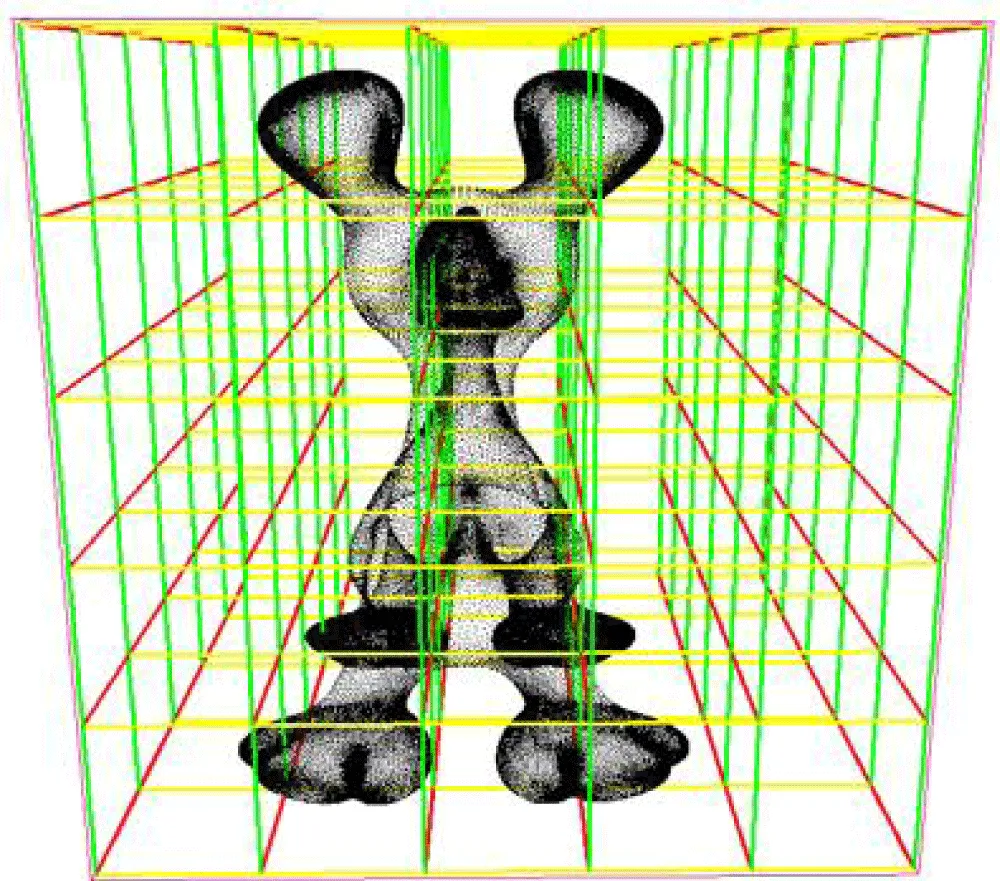
An implicit surface is defined by an analytical equation $F\mathrm{<mo\; stretchy="false">(</mo>}x\mathrm{,}y\mathrm{,}z\mathrm{<mo\; stretchy="false">)</mo><mo>=</mo>}C$ where $\mathrm{<mo\; stretchy="false">(</mo>}x\mathrm{,}y\mathrm{,}z\mathrm{<mo\; stretchy="false">)</mo>}$ belongs to a volume domain and C is a constant called “level” and the corresponding surface is a level set. A discrete representation of this surface is the data values of the underlying function, $F\mathrm{<mo\; stretchy="false">(</mo>}{x}_i\mathrm{,}{y}_j\mathrm{,}{z}_k\mathrm{<mo\; stretchy="false">)</mo>}$ , at the vertices $\mathrm{<mo\; stretchy="false">(</mo>}{x}_i\mathrm{,}{y}_j\mathrm{,}{z}_k\mathrm{<mo\; stretchy="false">)</mo>}$ of a 3D (Cartesian) grid, $1\le i\le n_i$ , $1\le j\le n_j$ and $1\le k\le n_k$ where $\mathrm{<mo\; stretchy="false">(</mo>}{n}_i\mathrm{,}{n}_j\mathrm{,}{n}_k\mathrm{<mo\; stretchy="false">)</mo>}$ are three integers defining the resolution of the grid, also implicitly representing the boundaries and so the (discrete) definition volume of the surface. Such a grid is often called a "voxel" grid, as shown in Figure 4.

Figure 4: A 3D Cartesian grid enclosing the point cloud model.

To compute function values $F\mathrm{<mo\; stretchy="false">(</mo>}{x}_i\mathrm{,}{y}_j\mathrm{,}{z}_k\mathrm{<mo\; stretchy="false">)</mo>}$  at each grid vertex P, we adopt a local approximation strategy based on point cloud data. For each vertex P, the m nearest neighbors ${\mathrm{<mo>\{</mo>}{Q}_i\mathrm{<mo>\}</mo>}}_{i\mathrm{<mo>=</mo>1}}^m$  in the point cloud are identified (in this paper m = 3 ) . Around each Q_i, a local quadratic surface is fitted:

${\phi }_i\mathrm{<mo\; stretchy="false">(</mo>}x\mathrm{,}y\mathrm{<mo\; stretchy="false">)</mo><mo>=</mo>}{a}_i{x}^2+b_{i}xy+c_i{y}^2\text{ (13)}$

where x and y are coordinates of P in a local coordinate system centered at Q_i. The distance from vertex $P\mathrm{<mo>=</mo><mo\; stretchy="false">(</mo>}x\mathrm{,}y\mathrm{,}z\mathrm{<mo\; stretchy="false">)</mo>}$ to the surface Q_i is computed as:

$d\mathrm{<mo\; stretchy="false">(</mo>}P\mathrm{,}{\phi }_i\mathrm{<mo\; stretchy="false">)</mo><mo>=</mo>}z-a_i{x}^2-b_{i}xy-c_i{y}^2\text{ (14)}$

The function value at P is then obtained through a weighted combination of these distances:

$F\mathrm{<mo\; stretchy="false">(</mo>}{x}_i\mathrm{,}{y}_j\mathrm{,}{z}_k\mathrm{<mo\; stretchy="false">)</mo><mo>=</mo>}{\displaystyle {\sum }_{i\mathrm{<mo>=</mo>1}}^m{\omega }_i}\cdot d\mathrm{<mo\; stretchy="false">(</mo>}P\mathrm{,}{\phi }_i\mathrm{<mo\; stretchy="false">)</mo>}\text{ (15)}$

The weight w_i for each surface is determined by the inverse distance magnitude, normalized by a harmonic normalization factor H:

${\omega }_i\mathrm{<mo>=</mo>}\frac{1}{\mathrm{<mo>|</mo>}d\mathrm{<mo\; stretchy="false">(</mo>}P\mathrm{,}{\phi }_i\mathrm{<mo\; stretchy="false">)</mo><mo>|</mo>}\cdot H}\mathrm{,}H\mathrm{<mo>=</mo>}{\displaystyle {\sum }_{i\mathrm{<mo>=</mo>1}}^m\frac{1}{\mathrm{<mo>|</mo>}d\mathrm{<mo\; stretchy="false">(</mo>}P\mathrm{,}{\phi }_i\mathrm{<mo\; stretchy="false">)</mo><mo>|</mo>}}}\text{ (16)}$

This formulation gives greater influence to surfaces closer to the point P, and ensures smooth interpolation across the grid.

Figures 5,6 illustrate this process. Figure 5 shows the topological relation between a grid vertex P and its neighboring point samples { Q_i }, while Figure 6 visualizes the local quadratic surface ϕ_I constructed at a point Q_i along with the projection of P onto the surface.

Figure 5: Schematic of voxel grid and local point sample geometry.

Figure 6: Visualization of the local quadratic surface ϕi near Qi and orthogonal distance from grid point P.

Applications

In this section, the proposed 3D reconstruction algorithm is applied to several point cloud datasets. For each case, we present the point cloud, the estimated normals, and the 3D reconstructed model. In certain examples, fine-resolution grids are employed to better capture geometric details during reconstruction.

The implicit surfaces are converted into 3D meshes using the PLOUGH3D software. The PLOUGH3D software generates the triangulation of a given level set of the implicit surface from a voxel grid. In addition, the software also generates the corresponding level curves in each plane z = zk. Several features are also available for optimization of the shape quality, simplification, and smoothing (roughness removal) of the resulting triangulation. The software also produces a closed surface of a given thickness around the imposed level. This kind of triangulation is particularly useful for surface 3D printing. The software includes several processing p hases:

• Analysis of the grid (minimum and maximum values and initialization of the parameter thresholds deduced from these values).
• Generation of the vertices of the triangulation on the edges of a 3D grid triangulation.
• Generation of the triangles of the triangulation.
• Extraction of the topology of the triangulation.
• Optimization of the shape quality of the triangulation.
• Simplification of the triangulation.
• Extraction of the connected components of the triangulation.
• Low frequency smoothing.
• Loading into memory and writing the resulting triangulation.

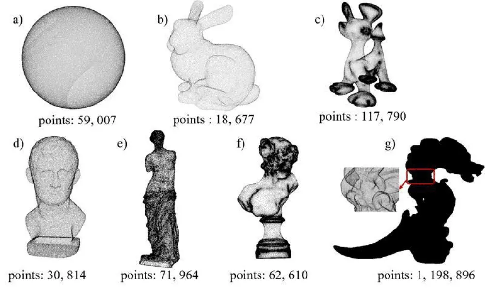
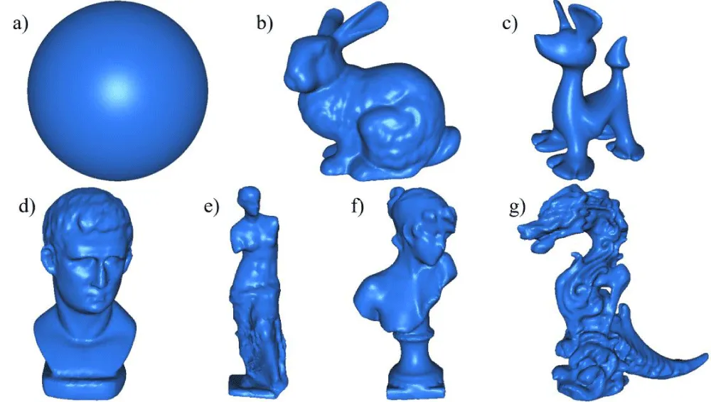
Figure 7 shows the point cloud data (from 18,667 points to 1,198,896 points), Figure 8 shows the corresponding normal estimation, and Figure 9 shows the reconstructed models.

Figure 7: Point clouds.

Figure 8: Normal estimation.

Figure 9: 3D reconstructed models.

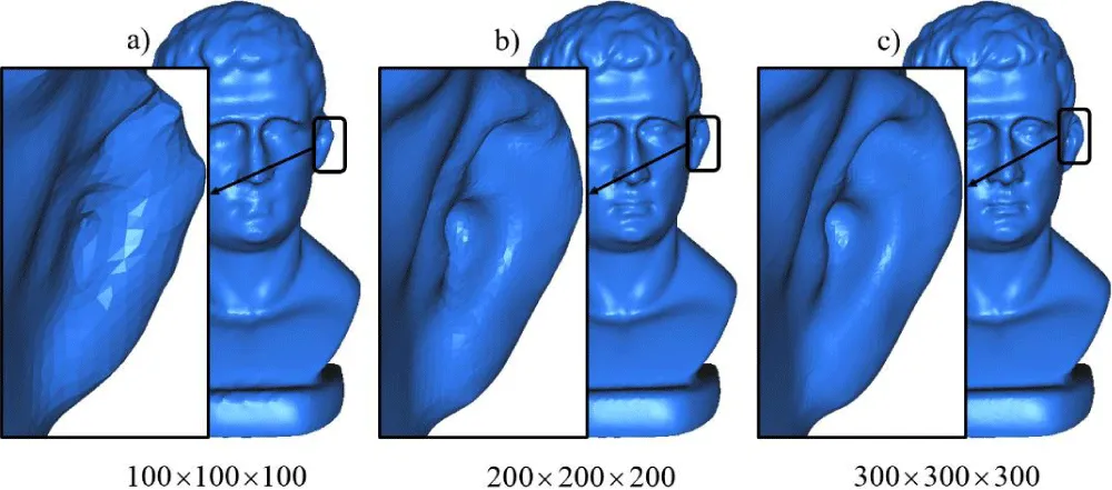
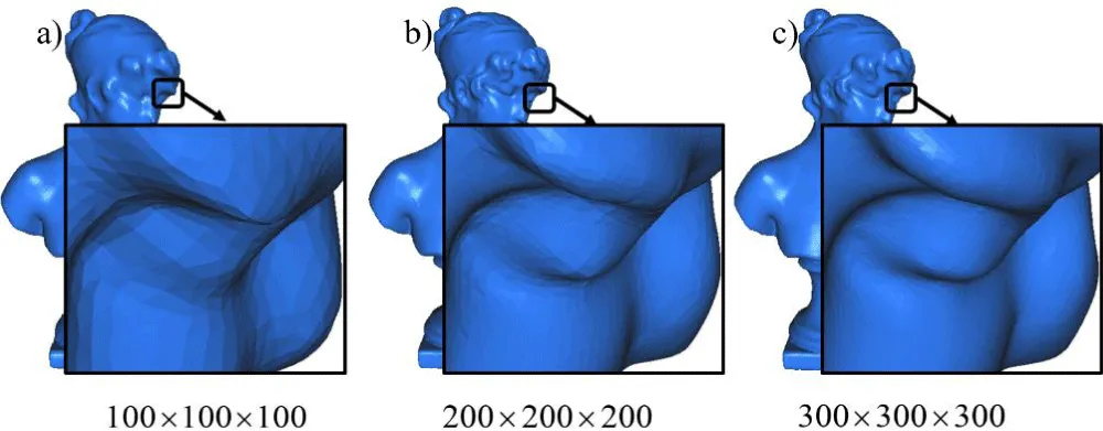
Using fine grids allows us to capture details on the surface (Figures 10-12).

Figure 10: Reconstructed models for 100×100×100, 200×200×200, and 300×300×300 grids.

Figure 11: Reconstructed models for 100×100×100, 200×200×200, and 300×300×300 grids.

Figure 12: Reconstructed models for 100×100×100, 200×200×200, and 300×300×300 grids.

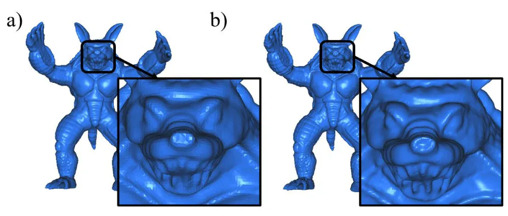
As demonstrated by the examples above, the proposed approach produces smoother geometric reconstructions across different levels of detail compared to existing methodologies. For illustration, Figure 13 presents a comparison between a reconstructions obtained using the Poisson method and one generated by our proposed approach.

Figure 13: Comparison with Poisson reconstruction.

Conclusion

In this paper, we propose a novel methodology for constructing discrete 3D models from point cloud data, based on implicit surface reconstruction. The approach addresses two key challenges: normal estimation and implicit surface definition. Several examples were presented to demonstrate the effectiveness and efficiency of the method.

Future extensions of this work include the incorporation of sharp edge features, where multiple normals must be considered, and the use of adaptive 3D grids for model construction. The latter would enable the capture of fine geometric details independently of dataset size, further enhancing the scalability and accuracy of the reconstruction process.

References

- Huang X, Mei G, Zhang J, Abbas R. A comprehensive survey on point cloud registration. arXiv [Preprint]. 2021; arXiv:2103.02690. Available from: https://doi.org/10.48550/arXiv.2103.02690
- Zhang T, Yuan H, Qi L, Zhang J, Zhou Q, Ji S. Point cloud Mamba: Point cloud learning via state space model. In: Proceedings of the AAAI Conference on Artificial Intelligence. 2025;39:10121–10130. Available from: https://doi.org/10.1609/aaai.v39i10.33098
- Chibane J, Alldieck T, Pons-Moll G. Implicit functions in feature space for 3D shape reconstruction and completion. In: Proceedings of the IEEE/CVF Conference on Computer Vision and Pattern Recognition. 2020;6970–6981. Available from: https://doi.org/10.1109/CVPR42600.2020.00700
- Choy CB, Xu D, Gwak J, Chen K, Savarese S. 3D-R2N2: A unified approach for single and multi-view 3D object reconstruction. In: Computer Vision – ECCV 2016: 14th European Conference on Computer Vision; 2016 Nov 11–14; Amsterdam, The Netherlands. Proceedings, Part VIII. Springer; 2016;628–644. Available from: https://arxiv.org/abs/1604.00449
- Carr JC, Beatson RK, Cherrie JB, Mitchell TJ, Fright WR, McCallum BC, et al. Reconstruction and representation of 3D objects with radial basis functions. In: Proceedings of the 28th Annual Conference on Computer Graphics and Interactive Techniques (SIGGRAPH). 2001; p. 67–76. Available from: https://doi.org/10.1145/383259.383266
- Nguyen TT, Nguyen QM, Liu XG, Ziggah YY. 3D object model reconstruction based on laser scanning point cloud data. In: International Symposium on Geoinformatics for Spatial Infrastructure Development in Earth and Allied Sciences. 2012. Available from: https://www.researchgate.net/publication/306278163_3D_OBJECT_MODEL_RECONSTRUCTION_BASED_ON_LASER_SC…
- Li X, Wang Y, Liu Y, Gao X, Song B. Qiyun Pagoda 3D model reconstruction based on laser cloud data. Surv Mapp. 2011;9:11–14.
- Boulch A. ConvPoint: Continuous convolutions for point cloud processing. Comput Graph. 2020;88:24–34. Available from: https://doi.org/10.48550/arXiv.1904.02375
- Brunetaud X, De Luca L, Janvier-Badosa S, Beck K, Al-Mukhtar M. Application of digital techniques in monument preservation. Eur J Environ Civ Eng. 2012;16(5):543–556. Available from: https://doi.org/10.1080/19648189.2012.676365
- Kwak E, Detchev I, Habib A, El-Badry M, Hughes C. Precise photogrammetric reconstruction using model-based image fitting for 3D beam deformation monitoring. J Surv Eng. 2013;139(3):143–155. Available from: https://doi.org/10.1061/(ASCE)SU.1943-5428.0000105
- Ren P, Wang W, Bai X. Reconstruction of Imperial University of Shanxi based on virtual reality technology. Comput Simul. 2012;29(11):20–23.
- Wang P, Wang Z, Xin S, Gao X, Wang W, Tu C. Restricted Delaunay triangulation for explicit surface reconstruction. ACM Trans Graph. 2022;41(5):1–20. Available from: https://doi.org/10.1145/3533768
- Lei H. OffsetOPT: Explicit surface reconstruction without normals. arXiv [Preprint]. 2025; arXiv:2503.15763. Available from: https://doi.org/10.48550/arXiv.2503.15763
- Berger M, Tagliasacchi A, Seversky LM, Alliez P, Guennebaud G, Levine JA, et al. A survey of surface reconstruction from point clouds. Comput Graph Forum. 2017;36(1):301–329. Available from: https://doi.org/10.1111/cgf.12802
- Ham H, Wesley J, Hendra H. Computer vision-based 3D reconstruction: A review. Int J Electr Comput Eng. 2019;9(4):2394–2402. Available from: https://doi.org/10.11591/ijece.v9i4.pp2394-2402
- Huang Z, Wen Y, Wang Z, Ren J, Jia K. Surface reconstruction from point clouds: A survey and a benchmark. IEEE Trans Pattern Anal Mach Intell. 2024. Available from: https://doi.org/10.1109/tpami.2024.3429209
- Lim SP, Haron H. Surface reconstruction techniques: A review. Artif Intell Rev. 2014;42(1):59–78. Available from: https://link.springer.com/article/10.1007/s10462-012-9329-z
- Zhao HK, Osher S, Fedkiw R. Fast surface reconstruction using the level set method. In: Proceedings of the IEEE Workshop on Variational and Level Set Methods in Computer Vision. 2001; p. 194–201. Available from: https://doi.org/10.1109/VLSM.2001.938900
- Kazhdan M, Hoppe H. Screened Poisson surface reconstruction. ACM Trans Graph. 2013;32(3):1–13. Available from: https://doi.org/10.1145/2487228.2487237
- Liu P, Zeng Z, Wang Q, Chen M, Zhang G. Geometry-enhanced implicit function for detailed clothed human reconstruction with RGB-D. arXiv [Preprint]. 2025; arXiv:2503.17921. Available from: https://doi.org/10.1049/cit2.70009
Save to Mendeley