Contraction and Periodic Orbits in Time-Periodic Filippov Systems?

Model and assumptions

Standing dimension. We formulate the framework for general n ∈N, although all main results in this paper are applied with n = 2 (planar systems).

Assumption 1 (Filippov system setup). Let T > 0 and $\mathbb{T}:=ℝ/T\mathbb{Z}$ denote time modulo T. Let $h\in C^1({ℝ}^n,ℝ)$ with ∇h(x) ̸= 0 for all x ∈ Σ, and define

$\text{Σ}:=\{x\in {ℝ}^n:h(x)=0\}, {\text{Ω}}^{\pm }:=\{x\in {ℝ}^n:h(x)\gtrless 0\}, n(x):=\frac{\nabla h(x)}{\parallel \nabla h(x)\parallel }.\text{ (4)}$

We assume Σ is the unique discontinuity manifold. Let $f:\mathbb{T}\times {ℝ}^n\to {ℝ}^n$ be T-periodic in t and C1 in x on each side of Σ, with restrictions

f±: = f|_T×_Ω±,   D_xf^±(t,x) := ∇_xf^±(t,x),            (5)

Both admit continuous one-sided extensions to Σ (including their Jacobians). The associated Filippov set-valued map is

$F(t,x):=\overline{co}\{\underset{\epsilon \to 0^{+}}{\text{lim}}f(t,x\pm \epsilon n(x))\},\text{ (6)}$

which coincides with f off Σ and convexifies f± on Σ. A Filippov solution is an absolutely continuous function x(·) such that

$\dot{x}(t)\in F(t,x(t)) \text{fora}.\text{e}. t\ge 0.\text{ (7)}$

Remark 1 (Single switching manifold). We restrict to a single codimension-one switching manifold Σ = {h = 0}; no additional or higher-codimension discontinuities are considered.

Weights, metric, and orbital derivatives. We introduce one-sided scalar weights

$W^{\pm }:\mathbb{T}\times {\text{Ω}}^{\pm }\to ℝ,\text{ (8)}$

(When switch counts N(t) are invoked later, they refer to the union of switching events of x(·) and y(·) on [0,t].) The orbital derivatives along f± are

A(t) := e^W(t,x(t)) ∥x(t) − y(t)∥,        ∥·∥ the Euclidean norm. (9)

(When switch counts N(t) are invoked later, they refer to the union of switching events of x(·) and y(·) on [0,t].) The orbital derivatives along f± are

DW(t,x) := ∂tW(t,x) + ∇xW(t,x) · f(t,x),             (10)

which extend continuously to Σ from each side. For compactness of notation, define

$W(t,x):=\{\begin{array}{ll}{W}^{+}(t,x),\hfill & x\in {\text{Ω}}^{+},\hfill \\ W^{-}(t,x),\hfill & x\in {\text{Ω}}^{-},\hfill \end{array} \mathcal{D}W(t,x):=\{\begin{array}{ll}\mathcal{D}{W}^{+}(t,x),\hfill & x\in {\text{Ω}}^{+},\hfill \\ \mathcal{D}{W}^{-}(t,x),\hfill & x\in {\text{Ω}}^{-}.\hfill \end{array}\text{ (11)}$

On Σ, we record the jumps

[W](t,x) := W+(t,x) − W−(t,x),    [DW](t,x) := DW+(t,x) −DW−(t,x).   (12)

Sliding objects. On a sliding region Σ_slide ⊂ Σ, the Filippov sliding vector field f_slide(t,x) is defined as the unique convex combination

f_slide(t,x) = αf+(t,x) + (1 − α)f−(t,x),         α ∈ [0,1],

such that n(x)⊤f_slide(t,x) = 0, ensuring consistency with the Filippov set F(t,x). We fix a consistent trace W_Σ and introduce the tangential gradient ∇⊤ := (I-n (x)n(x)⊤)∇_x, and the sliding orbital derivative

D_ΣW(t,x) := ∂_tW_Σ(t,x) + ∇⊤W_Σ(t,x) · f_slide(t,x).            (13)

Clarke rates and the symmetric part. For any matrix A, write $S(A):=\frac{1}{2}(A+A^{\top })$ . The Clarke

n^o

${\partial }_{C}f(t,x):=co\{\underset{k\to \infty }{\text{lim}}{D}_{x}f(t_k,x_k): (t_k,x_k)\to (t,x), D_{x}f(t_k,x_k) \text{exists}\},$

and we define the maximal symmetric contraction rate

${\lambda }_{\text{max}}^{Cl}(t,x):=\underset{A\in {\partial }_{C}f(t,x)}{\text{sup}}{\lambda }_{\text{max}}(S(A)).\text{ (14)}$

On sliding arcs, we analogously set

${\lambda }_{\text{max}}^{Cl}(t,x;f_{\text{slide}}):=\underset{A\in {\partial }_C{f}_{\text{slide}}(t,x)}{\text{sup}}{\lambda }_{\text{max}}(S(A)).\text{ (15)}$

Off Σ, the generalized Jacobian reduces to the classical Jacobian, ∂_Cf(t,x) = {D_xf(t,x)}.

Assumption 2 (Global structural and contraction conditions). Let K ⊂ Rⁿ be compact and forward-invariant for the Filippov flow. We assume:

(A1) Time-periodicity and regularity: f is T-periodic in t, C¹ in x on K \ Σ, with continuous one-sided extensions (and Jacobians) to Σ.

(A2) Contraction off Σ: $\mathcal{D}W(t,x)+{\lambda }_{\text{max}}^{Cl}(t,x) \le -\nu \text{forsome}\nu >0.$

 (A3) Weighted jump contraction: There exists ϵ_jump > 0 such that for any crossing time t₀ of Σ (for a pair of Filippov solutions in K),

$A(t_0^{+}) \le e^{-{ϵ}_{\text{jump}}} A(t_0^{-}).$

(A4) Contraction on sliding: For (t,x) ∈ Σ_slide,

${\mathcal{D}}_{\text{Σ}}W(t,x)+{\lambda }_{\text{max}}^{Cl}(t,x;f_{\text{slide}}) \le -\nu ,$

And repelling sliding is excluded.

(A5) Dwell-time / no Zeno: There exists τ > 0 such that the time between consecutive crossings of Σ along any Filippov solution in K is at least τ.

Remark 2 (Initial conditions on Σ). If x₀ ∈ Σ_slide, the trajectory evolves according to f_slide, and contraction is determined by the sliding dynamics. In contrast, if x0 lies in a crossing region, the trajectory immediately enters one of the domains Ω±, where contraction follows the smooth dynamics.

Lemma 1 (Local-to-global contraction). Let K ⊂Rⁿ be compact, convex, and forward-invariant. Suppose there exist δ > 0, ν > 0, C > 0 such that for all x₀, y₀ ∈ K with ∥x₀ − y₀∥ < δ,

∥ϕ(t,x₀) − ϕ(t,y₀)∥ ≤ C e−νt ∥x₀ − y₀∥,     ∀t ≥ 0.

Then there exists C′ > 0 (depending only on C, δ, K) such that for all x₀, y₀ ∈ K and t ≥ 0,

∥ϕ(t,x₀) − ϕ(t,y₀)∥ ≤ C′ e−νt ∥x₀ − y₀∥.

The same conclusion holds if the local inequality is stated in any norm uniformly equivalent to the Euclidean norm on K (e.g., the weighted metric defined via W).

Proof. Fix x₀, y₀ ∈ K and, to avoid any ambiguity arising from possible nonuniqueness of Filippov solutions, fix once and for all a single–valued selection

$\varphi : [0,\infty )\times K\to K, (t,z)\mapsto \varphi (t,z),$

of Filippov trajectories (if solutions are unique, ϕ is the flow). The local hypothesis is assumed to hold for this selection. The claim is trivial when x₀ = y₀, so assume x₀ ≠ y₀.

Step 1: Partition of the straight segment inside K. Since K is convex, the straight segment

γ(s):= (1 − s)x₀ + sy₀, s ∈ [0,1],

is contained in K. Choose

$m:=\text{max}\{1, \lfloor 2\parallel y_0-x_0\parallel /\delta \rfloor \}, s_j:=\frac{j}{m} (j=0,1,\dots ,m), z_j:=\gamma (s_j).$

Then z_j ∈ K for all j and

$\parallel z_{j+1}-z_j\parallel =\frac{\parallel y_0-x_0\parallel }{m}\le \frac{\delta }{2}<\delta (j=0,\dots ,m-1).$

Step 2: Propagation of the local estimate along the chain. By forward invariance of K, ϕ(t,z_j) ∈ K for all t ≥ 0 and all j. Hence, the local contraction inequality applies to each adjacent pair (z_j, z_{j + 1}):

$\parallel \varphi (t,z_{j+1})-\varphi (t,z_j)\parallel \le C e^{-\nu t} \parallel z_{j+1}-z_j\parallel \forall t\ge 0.\text{ (16)}$

Summing (16) over j = 0,...,m − 1 and using the triangle inequality yields

$\parallel \varphi (t,y_0)-\varphi (t,x_0)\parallel \le {\displaystyle \sum }_{j=0}^{m-1}\parallel \varphi (t,z_{j+1})-\varphi (t,z_j)\parallel \le C e^{-\nu t}{\displaystyle \sum }_{j=0}^{m-1}\parallel z_{j+1}-z_j\parallel .$

Because γ is a straight segment, the polygonal length equals the chord length,

${\displaystyle \sum }_{j=0}^{m-1}\parallel z_{j+1}-z_j\parallel =\parallel y_0-x_0\parallel ,$

and therefore

∥ϕ(t,y₀) − ϕ(t,x₀)∥ ≤ C e^−νt ∥y₀ − x₀∥     ∀t ≥ 0.

This establishes the desired global bound with C′ = C in the Euclidean norm.

Step 3: Uniformly equivalent norms. Suppose instead that the local inequality is stated in a norm ∥·∥∗ uniformly equivalent to the Euclidean norm on K, i.e., there exist constants 0 < c₁ ≤ c₂ < ∞ such that

c₁∥v∥ ≤ ∥v∥∗ ≤ c₂∥v∥     ∀v ∈Rⁿ.

Repeating Step 2 with ∥·∥∗ in place of ∥·∥ gives

$\parallel \varphi (t,y_0)-\varphi (t,x_0){\parallel }_{\text{*}}\le C{e}^{-\nu t}{\displaystyle \sum }_{j=0}^{m-1}\parallel z_{j+1}-z_j{\parallel }_{\text{*}}$

Using norm equivalence on both sides and on the increments,

$\parallel \varphi (t,y_0)-\varphi (t,x_0)\parallel \le \frac{1}{c_1}\parallel \varphi (t,y_0)-\varphi (t,x_0){\parallel }_{\text{*}} \le \frac{C}{c_1} e^{-\nu t}{\displaystyle \sum }_{j=0}^{m-1}\parallel z_{j+1}-z_j{\parallel }_{\text{*}}$

$\le \frac{C c_2}{c_1} e^{-\nu t}{\displaystyle \sum }_{j=0}^{m-1}\parallel z_{j+1}-z_j\parallel = \frac{C c_2}{c_1} e^{-\nu t} \parallel y_0-x_0\parallel .$

Thus, the conclusion holds with C′ = (c₂/c₁)C.

Remarks on assumptions. Convexity ensures γ([0,1]) ⊂ K; forward invariance ensures ϕ(t, z_j) ∈ K for all t ≥ 0, so the local estimate is valid along the entire chain. Compactness of K is not used explicitly in the inequalities, but it is standard for well-posedness and for bounding constants. The choice of m guarantees each link length is strictly less than δ, activating the local hypothesis on every adjacent pair.            

Theorem 1 (Transfer from weighted to Euclidean contraction). Let W: T × K →R be continuous and bounded, and define

$M:=\underset{(t,x)\in \mathbb{T}\times K}{\text{sup}}|W(t,x)|<\infty .$

Suppose x(·),y(·) are Filippov solutions with x(0),y(0) ∈ K \ Σ such that

A(t) := e^W(t,x(t)) ∥x(t) ^{− y(t)}∥ ≤ A(0)e−νt      ∀t ≥ 0.

Then, for all t ≥ 0,

Proof. By forward invariance of K, x(t),y(t) ∈ K for all t ≥ 0. Since W is bounded on T× K, we have

e−M ≤ eW(t,x(t)) ≤ eM,              t ≥ 0. (17)

∥x(t) − y(t)∥ ≤ e^MA(t), t ≥ 0,

at the initial time,

A(0) = e^W(0,x(0))∥x(0) − y(0)∥ ≤ e^M∥x(0) − y(0)∥.

Using the assumed decay A(t) ≤ A(0)e−νt, we combine these inequalities:

$\parallel x(t)-y(t)\parallel \le e^{M}A(t) \le e^{M}A(0)e^{-\nu t} \le e^M(e^M\parallel x(0)-y(0)\parallel )e^{-\nu t}.$

Thus,

∥x(t) − y(t)∥ ≤ e^2M e^−νt ∥x(0) − y(0)∥,

which is the desired estimate.

Theorem 2 (Average contraction under a bounded switching rate). Let K ⊂ Rⁿ be compact and forward-invariant, and let x(·),y(·) be Filippov solutions with values in K. Define the weighted distance

A(t) := e^W(t,x(t)) ∥x(t) − y(t)∥,

where ∥·∥ is the Euclidean norm and W is bounded on T× K. Assume:

(i) Smooth/sliding contraction: On any interval free of switching events, A(·) is absolutely continuous and satisfies

$\dot{A}(t)\le -\nu A(t) \text{fora}.\text{e}. t,$

for some ν > 0.

(ii) Jump update: At each switching time, tk,

$A(t_k^{+}) \le e^{\kappa } A(t_k^{-}),$

for some κ ∈R.

(iii) Switching-rate bound: The cumulative number of switches up to time t satisfies

N(t) ≤ ρt + N₀,             t ≥ 0,

for some ρ ≥ 0 and N₀ ∈ N₀.

Then, for all t ≥ 0,

A(t) ≤ A(0)e−(ν−ρκ)t eκN0.

Moreover, if

$M:=\underset{(t,x)\in \mathbb{T}\times K}{\text{sup}}|W(t,x)|<\infty ,$

then

∥x(t) − y(t)∥ ≤ e2^M+κN0 e^{−(ν−ρκ)t} ∥x(0) − y(0)∥,       t ≥ 0.

Proof. Let {t_k}_k≥1 denote the (strictly increasing) sequence of switching times for the pair (x(·),y(·)), with t₀:= 0 and t_N(t)+1:= t. By assumption (iii), N(t) < ∞ for each finite t, so no Zeno accumulation occurs.

Step 1 (Decay on event-free intervals). On any interval [s,u] containing no switch, assumption (i) and Grönwall’s inequality give

$A(u^{-}) \le e^{-\nu (u-s)} A(s^{+}).\text{ (18)}$

In particular,

$A(t_{k+1}^{-}) \le e^{-\nu (t_{k+1}-t_k)} A(t_k^{+}) (k=0,1,\dots ,N(t)).$

^{Step 2 (Jump updates)}. A(t) each switch, t_k, assumption (ii) yields

$A(t_k^{+}) \le e^{\kappa }A(t_k^{-}).$

A(t+k ) ≤ eκA(t−k ).

Step 3 (Concatenation). Alternating the decay estimates with the jump updates and multiplying along the chain gives

A(t+) ≤ e^−νt e^κN(t) A(0⁺).

If t is not a switching time, then A(t) = A(t+); if t is a switching time, then the last update has already been accounted for. Thus

A(t) ≤ A(0)e^−νt e^κN(t),   t ≥ 0.

Step 4 (Average rate). Using assumption (iii), N(t) ≤ ρt + N0, we obtain

$A(t) \le A(0) e^{-(\nu -\rho \kappa )t} e^{\kappa N_0}, t\ge 0.$

Step 5 (Conversion to Euclidean norm). Since |W(t,x)|≤ M, we have

∥x(t) − y(t)∥ ≤ e^MA(t), A(0) ≤ e^M∥x(0) − y(0)∥.

Substituting into the bound for A(t) yields

$\parallel x(t)-y(t)\parallel \le e^{2M+\kappa N_0} e^{-(\nu -\rho \kappa )t} \parallel x(0)-y(0)\parallel ,$

as claimed.

Application

We illustrate the theory with a classical mechanics example: a mass–spring–damper system subject to Coulomb friction and periodic forcing. Let x = (q,v), where q denotes displacement and v velocity. The parameters are the natural frequency ω0, damping ratio ζ, friction magnitude µg, forcing amplitude F, and forcing frequency Ω. The dynamics are

$\dot{q}=v, \dot{v}=-{\omega }_0^{2}q-2\zeta {\omega }_{0}v-\mu g \text{sgn}(v)+F\text{cos}(\text{Ω}t),\text{ (19)}$

interpreted in the Filippov sense on the switching manifold Σ = {v = 0}. Sliding (sticking) occurs on

${\text{Σ}}_{\text{slide}}=\{(t,q,0): |-{\omega }_0^{2}q+F\text{cos}(\text{Ω}t)|\le \mu g\},$

With v˙ = 0 enforced by an internal friction force. The tangential flow is q˙ = 0, so q remains constant during sticking. Away from Σ, the right-hand side of (19) is C¹ and piecewise affine.

Parameters.

Fix

ω₀ = 1,             ζ = 1,     µg = 0.6,               F = 0.4, Ω = 1    (T = 2π).

These values guarantee sticking in part of each period ( $|-{\omega }_0^{2}q+F\text{cos}t|\le 0.6$ holds for a nonempty interval) and at most two stick–slip transitions per period. Thus

$N(t) \le \rho t+N_0, \rho =\frac{2}{T}=\frac{1}{\pi }.$

Contraction of Σ (Assumption 2(A2)). On either side of Σ, the Jacobian of (19) is constant,

$J=\left[\begin{array}{ll}0\hfill & 1\hfill \\ -{\omega }_0^2\hfill & -2\zeta {\omega }_0\hfill \end{array}\right]=\left[\begin{array}{ll}0\hfill & 1\hfill \\ -1\hfill & -2\hfill \end{array}\right].$

Choose the quadratic weight.

$P=\left[\begin{array}{ll}\frac{3}{2}\hfill & \frac{1}{2}\hfill \\ \frac{1}{2}\hfill & \frac{1}{2}\hfill \end{array}\right]\text{}>\text{}0,$

This solves the Lyapunov inequality

J^⊤P + PJ = −I.

Writing ∥x∥P := (x^⊤Px)^1/2 for the associated norm, we compute

$\frac{d}{dt} \delta x^{\top }P \delta x = \delta x^{\top }(J^{\top }P+PJ)\delta x \le - \parallel \delta x{\parallel }^2 \le -\frac{1}{{\lambda }_{\text{max}}(P)} \delta x^{\top }P \delta x,$

So the contraction rate is

$\nu =\frac{1}{2{\lambda }_{\text{max}}(P)}=\frac{1}{2(1+\frac{\sqrt{2}}{2})}\approx 0.293$

In the P- metric.

Contraction on sliding (Assumption 2(A4)).

On Σslide, the tangential dynamics reduce to q˙ = 0, so separations tangent to Σ are nonexpanding. Together with dissipative normal dynamics enforcing v˙ = 0, the sliding vector field is contracting in the same quadratic metric.

Jump updates and average-rate bound (Assumption 2(A3)). Introduce a piecewise-constant scalar weight with traces.

W+ = α,           W− = −α,               α = 0.05.

Then [W] = 2α, and the weighted distance

A(t) = e^W(t,x)∥x − y∥P

incurs a multiplicative factor eκ with κ = 2α = 0.1 at each transversal crossing of Σ. With

N(t) ≤ ρt + N0 and ρ = 1/π, Theorem 2 yields the effective rate

${\nu }_{\text{eff}}=\nu -\rho \kappa \approx 0.293-\frac{0.1}{\pi } \approx 0.261 > 0,$

so average exponential contraction persists despite switching.

Transfer to Euclidean decay (Theorem 1).

Since |W|≤ α on T× K, we have ∥W∥∞ = α. Thus, the weighted and Euclidean distances are uniformly equivalent up to factors e±α. Theorem 1 transfers exponential decay to the Euclidean norm with the same rate νeff, up to fixed multiplicative constants.

Local-to-global and periodic orbit (Lemma 1). The local differential estimate above, together with the convexity and forward invariance of a rectangular set

K = {(q,v) : |q|≤ Q, |v|≤ V },

(chosen via a standard energy estimate) activates Lemma 1 and yields global incremental contraction on K. For T-periodic forcing, the stroboscopic map ϕ(T,·) is a contraction on K; hence, by Banach’s fixed-point theorem, there exists a unique T-periodic Filippov solution in K, exponentially orbitally stable with rate νeff.

Numerical illustration

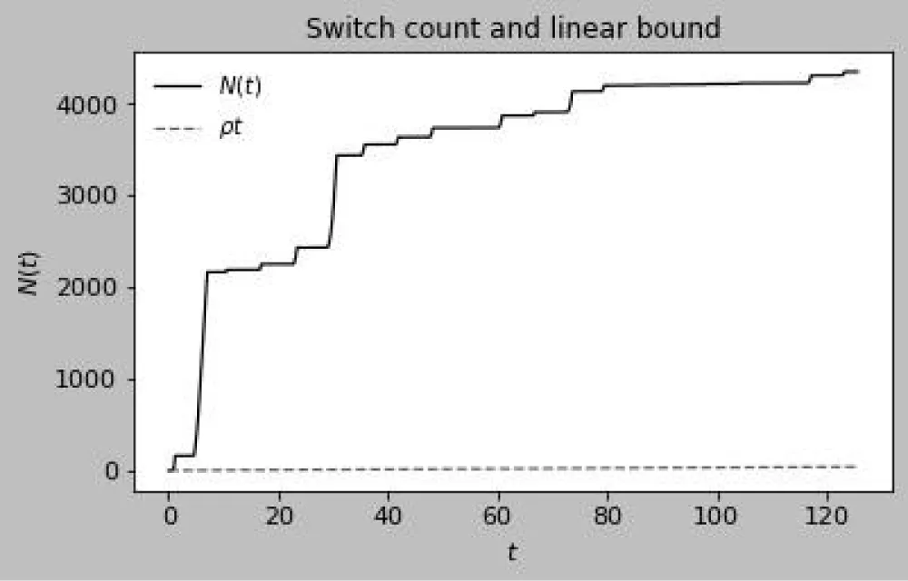
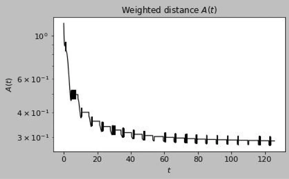
We verified the theoretical predictions by simulating pairs of trajectories using an event-driven scheme with zero-crossing detection and explicit enforcement of sliding motion. The numerical results confirm the following points: (i) distances between distinct initial conditions decay exponentially at rate close to −νeff, both in the weighted and Euclidean metrics; (ii) phase portraits display alternating slip and sliding segments, converging to a unique T-periodic orbit as predicted by the contraction of the stroboscopic map; and (iii) the observed number of switches grows linearly with slope approximately 1/π, in agreement with the assumed bound. All parameters (P,ν,κ,ρ,M) are explicit, demonstrating that the proposed framework can be verified and visualized directly on a classical mechanical system.

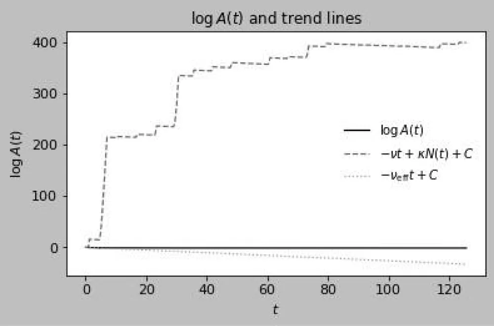
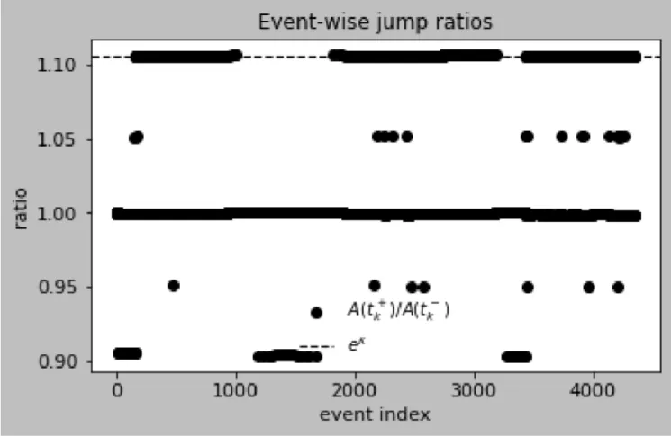
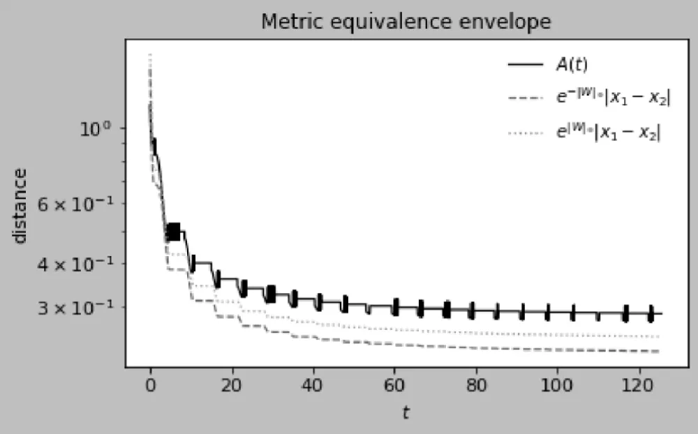
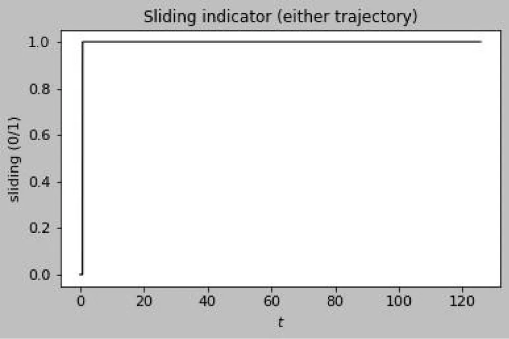
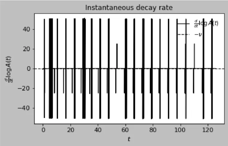
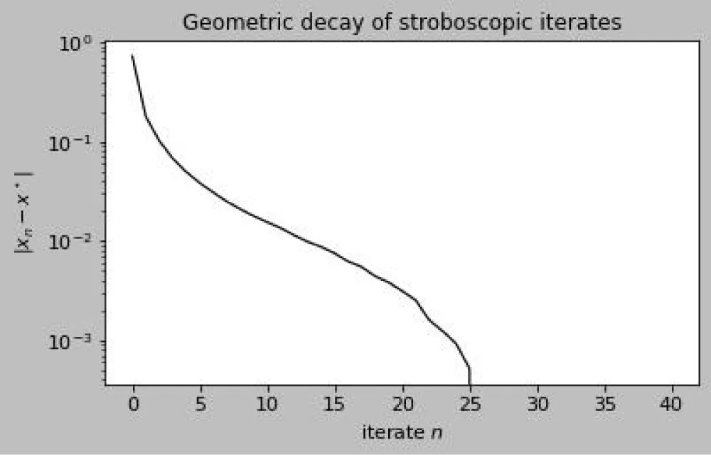
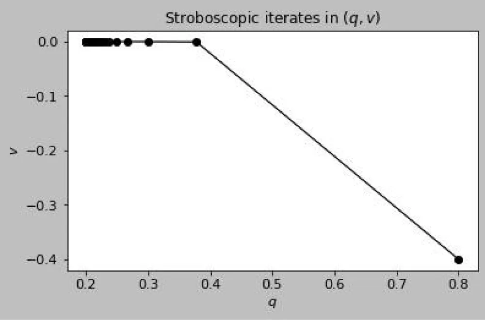
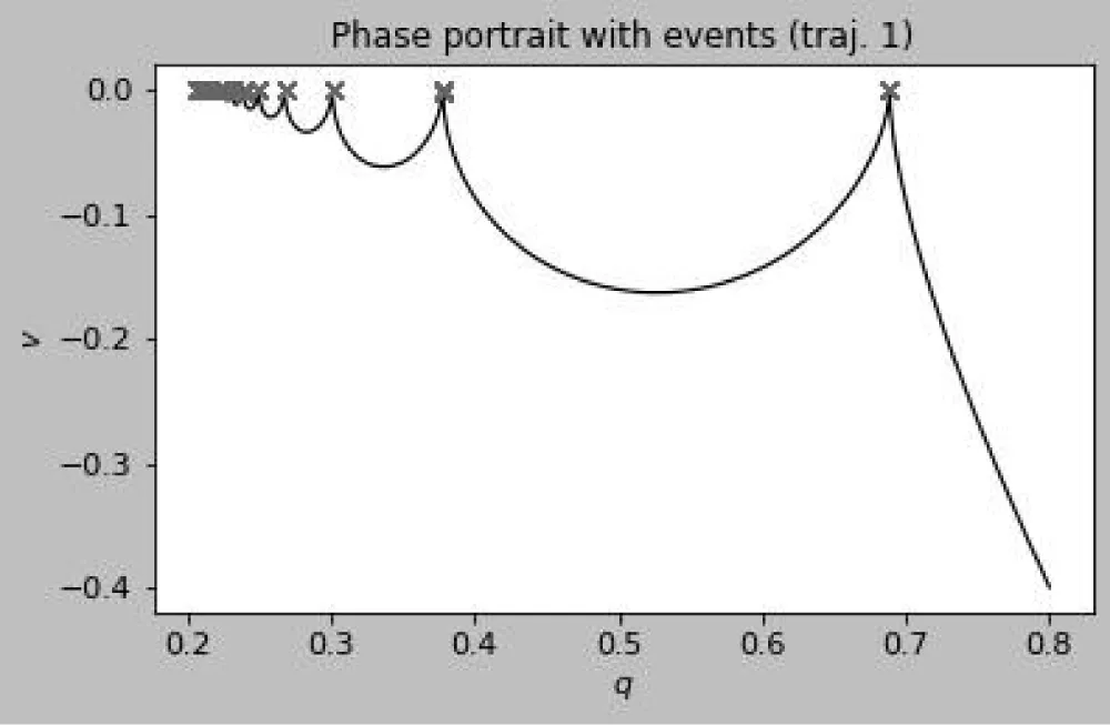
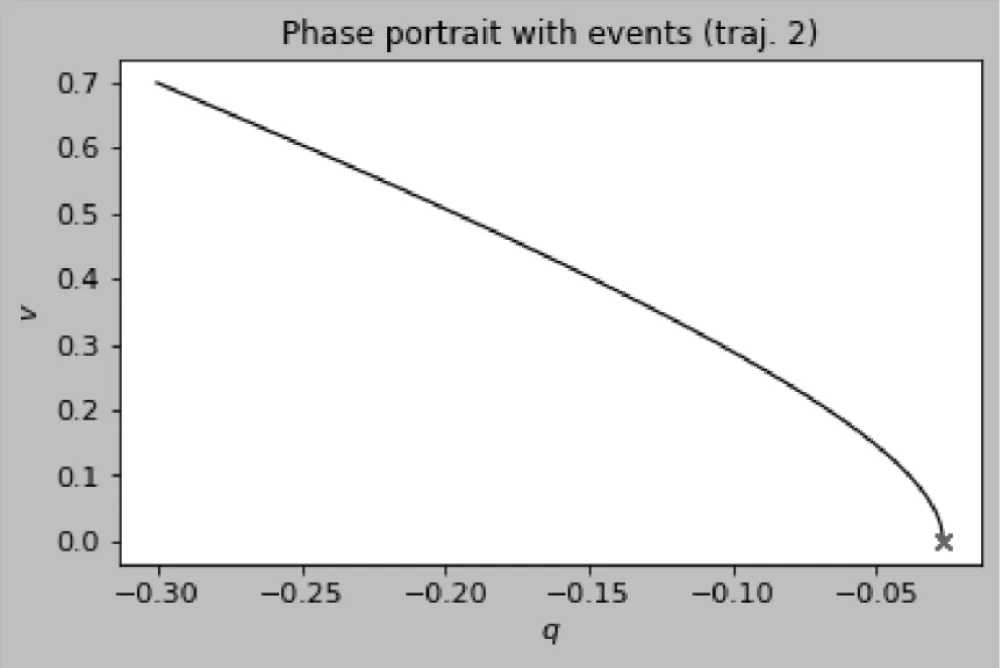
Discussion of figures. The numerical results are consistent with the theoretical framework and illustrate its key mechanisms. Figure 1 shows the weighted distance A(t) between two trajectories on a semilog scale: the staircase profile reflects the interplay between continuous contraction and discrete jumps, with exponential decay at rate $\nu =\frac{1}{2{\lambda }_{\text{max}}(P)}$ between events and multiplicative factors e^κ applied at transversal crossings of the switching manifold, yielding an overall downward trend that anticipates the effective rate −νeff. This interpretation is reinforced in Figure 2, where logA(t) closely follows the theoretical bounds –νt + κN(t) + C and −ν_efft + C after a short transient, with slope matching the predicted −ν_eff = ν-ρκ. Figures 3 and 4 examine the event structure in more detail: jump ratios remain bounded by eκ, confirming Assumption 2(A3), while the cumulative switch count grows essentially linearly and respects the assumed envelope N(t) ≤ ρt + N0, with observed deviations attributable to numerical chatter near the manifold rather than genuine crossings. Metric equivalence is illustrated in Figure 5, where A(t) remains sandwiched between the Euclidean distances scaled by e±∥W∥∞, validating the transfer of contraction to the standard norm as formalized in Theorem 1. Sliding intervals, highlighted in Figure 6, demonstrate the applicability of Assumption 2(A4): during sticking, the tangential flow is nonexpansive while normal dynamics dissipate, ensuring contraction even in the absence of motion along Σ. The instantaneous decay rate shown in Figure 7 further corroborates the analysis: between events, dtd logA(t) remains below −ν, while discrete spikes at switching instants are bounded by κN(t), producing the average contraction profile. The long-term behavior is captured in Figures 8–9, where contractivity of the stroboscopic map $x\mapsto \varphi (T,x)$ is evident from the geometric decay of distances between iterates and their convergence to a unique fixed point, corresponding to the unique exponentially stable T-periodic Filippov solution guaranteed by Banach’s theorem. Finally, the phase portraits in Figures 10–11 illustrate the qualitative stick–slip dynamics: trajectories undergo alternating slip and sliding episodes yet converge rapidly to the same periodic orbit, visually confirming the incremental contraction and uniqueness results established in Section 2 [20-30].

Figure 1: Weighted distance A(t) on a semilog scale. Step-like increases correspond to switching across Σ, where the multiplicative jump e^κ is applied (κ = 0.1). Between events, the smooth/sliding dynamics contract at a rate $\nu =\frac{1}{2{\lambda }_{\text{max}}(P)}$ . Model and parameters as stated above.

Figure 1: Trend verification for Theorem 2. We plot logA(t) together with the theoretical upper bounds −νt+κN(t)+C and −νefft+C, where N(t) counts switches (union over both trajectories) and νeff = ν-ρκ with ρ = 1/π.

Figure 3: Event-wise jump ratios $A(t_k^{+})/A(t_k^{-})$ at detected switching times t_k. The dashed line shows e^κ with κ = 0.1. This tests the jump-contraction hypothesis (A3) encoded in the weight W.

Figure 4: Switch counter N(t) and the linear bound ρt with ρ = 1/π. This verifies the average-rate assumption used in Theorem 2 to obtain ν_eff = ν − ρκ.

Figure 5: Metric-equivalence envelope for Theorem 1. The weighted distance A(t) lies between e^{−∥W∥∞}∥x1(t) − x2(t)∥ and e^∥W∥∞∥x1(t) − x2(t)∥ with ∥W∥∞ = α = 0.05, showing transfer of decay from the weighted metric to the Euclidean norm.

Figure 6: Sliding indicator (1 when either trajectory satisfies v = 0 and $|-{\omega }_0^{2}q+F\text{cos}(\Omega t)|\le \mu g|$ or Contraction on sliding segments follows from (A4), as the tangential sliding field is nonexpansive in the chosen metric while normal dynamics enforce sticking.

Figure 7: Finite-difference estimate of $\frac{d}{dt}\text{log}A(t)$ with reference line at −ν. Between jumps, the instantaneous decay does not exceed −ν, consistent with (A2) off Σ and (A4) on Σ_slide; positive spikes correspond to discrete jump updates.

Figure 8: Contraction of the stroboscopic map. Iterates xn+1 = ϕ(T,xn) satisfy ∥xn − x⋆∥ decaying geometrically (semilog plot), confirming contractivity of ϕ(T,·) on the invariant set and the existence/uniqueness of a T-periodic Filippov orbit via Banach’s fixed-point theorem.

Figure 9: Stroboscopic iterates in phase space (q,v). The sequence xn converges to a fixed point x⋆ of the return map, corresponding to a T-periodic solution of the Filippov system.

Figure 10: Phase portrait of trajectory 1 with event markers (crosses) at zero crossings of v. Sliding occurs along Σ = {v = 0} when the Filippov condition holds; slip arcs follow the piecewise-smooth vector field with Coulomb friction.

Figure 11: Phase portrait of trajectory 2 with event markers. Together with Figure 10, this illustrates how different initial conditions converge under the combined smooth/sliding contraction and bounded switching penalties.

Conclusion

We have developed a unified, saltation-free contraction framework for time-periodic Filippov systems on compact forward-invariant sets with a single codimension-one switching manifold. The framework employs a weighted distance that consistently incorporates smooth flow, sliding motion, and jump updates within a single analytic calculus. Within this setting, we established: (i) a local-to-global principle for incremental contraction (Lemma 1); (ii) a transfer theorem showing that exponential decay in the weighted metric implies Euclidean decay with explicit constants (Theorem 1); and (iii) an average-rate result quantifying the impact of switching frequency on effective contraction rates (Theorem 2). A canonical mass–spring–damper with Coulomb friction demonstrated the verifiability of the assumptions, the explicitness of the constants, and the visualization of the predicted decay rates.

The methodology is deliberately saltation-free: discontinuous events are captured as multiplicative updates of the weighted distance, while contraction away from the manifold is expressed using Clarke’s generalized Jacobian, and sliding dynamics are treated via the tangential Filippov flow. This results in explicit, computable constants and rates that allow for practical certification in physics- and engineering-motivated models. Natural extensions include the treatment of multiple switching manifolds, higher-dimensional dynamics, robustness under perturbations, and data-driven design of admissible weights and contraction metrics.

A complementary and promising direction is to integrate spectral approaches with the present framework. Stiefenhofer [26, 27] has recently advanced a spectral contraction framework for planar Filippov systems, proving the existence and exponential stability of nonsmooth periodic orbits via spectral properties of the Poincaré map. Combining such spectral techniques with the explicit metric-based analysis developed here offers the prospect of a more comprehensive theory, capable of addressing higher-dimensional settings, multiple switching manifolds, and nonconvex invariant sets. Pursued together, these approaches promise to significantly expand the scope and applicability of contraction methods for nonsmooth dynamics across mathematics, physics, engineering, and the applied sciences.

References

1. di Bernardo M, Budd CJ, Champneys AR, Kowalczyk P. Piecewise-smooth dynamical systems: theory and applications. Springer; 2008. Available from: http://dx.doi.org/10.1109/MCS.2008.929164
2. Kunze M. Non-smooth dynamical systems. Lecture Notes in Mathematics, vol. 1744. Springer-Verlag; 2000. Available from: https://link.springer.com/book/10.1007/BFb0103843
3. Giesl P. Existence of periodic orbits in nonsmooth differential equations using contraction mappings. J Math Anal Appl. 2005;306(1):203–18. Available from: http://dx.doi.org/10.1002/zamm.200310164
4. Leine RI, van Campen DH, van de Vrande BL. Stick–slip vibrations induced by alternate friction models. Nonlinear Dyn. 2000;23(2):105–30. Available from: http://dx.doi.org/10.1177/1461348419853658
5. Leine RI, van Campen DH, van de Vrande BL. Stick–slip vibrations induced by alternate friction models. Nonlinear Dyn. 2000;23(2):105–30. https://pure.tue.nl/ws/files/1478861/605090.pdf
6. Guardia M, Seara TM, Teixeira MA. Generic bifurcations of low codimension of planar Filippov systems. J Differ Equations. 2010;250(4):1967–2023. Available from: https://doi.org/10.1016/j.jde.2010.11.016
7. Li Y, Dankowicz H. Bifurcation analysis of stick–slip oscillations in discontinuous dynamical systems. Nonlinear Dyn. 2021;103(2):1355–74.
8. Stiefenhofer P, Giesl P. Switching regimes in economics: the contraction mapping and the ω-limit set. Appl Math. 2019;10(7):513–20. Available from: https://doi.org/10.4236/am.2019.107035
9. Stiefenhofer P, Giesl P. A global stability theory of nonsmooth periodic orbits: example I. Appl Math Sci. 2019;13(11):511–20. Available from: https://www.m-hikari.com/ams/ams-2019/ams-9-12-2019/p/stiefenhoferAMS9-12-2019-1.pdf
10. Stiefenhofer P. Economic stability of non-smooth periodic orbits in the plane: omega limit sets Part I. Nonlinear Anal Differ Equ. 2020;8(1):41–52. Available from: https://www.m-hikari.com/nade/nade2020/1-2020/p/stiefenhoferNADE1-2020-1.pdf
11. Stiefenhofer P. Economic stability of non-smooth periodic orbits in the plane: omega limit sets Part II. Nonlinear Anal Differ Equ. 2020;8(1):53–65. Available from: https://www.m-hikari.com/nade/nade2020/1-2020/p/stiefenhoferNADE1-2020-2.pdf
12. Pavlov A, Pogromsky A, van de Wouw N, Nijmeijer H. Convergent dynamics: a tribute to Boris Pavlovich Demidovich. Syst Control Lett. 2004;52(3–4):257–61. Available from: http://dx.doi.org/10.1016/j.sysconle.2004.02.003
13. Itō F. A Filippov solution of a system of differential equations with discontinuous right-hand side. Econ Lett. 1979;4:349–54. Available from: https://ideas.repec.org/a/eee/ecolet/v4y1979i4p349-354.html
14. Stiefenhofer P, Giesl P. Economic periodic orbits: a theory of exponential asymptotic stability. Nonlinear Anal Differ Equ. 2019;7(1):9–16. Available from: https://www.m-hikari.com/nade/nade2019/1-4-2019/p/stiefenhoferNADE1-4-2019.pdf
15. Dieci L, Elia C, Lopez L. Networks of piecewise-smooth Filippov systems and stability of synchronous periodic orbits. Discret Contin Dyn Syst B. Forthcoming 2025;30:6. https://www.aimsciences.org/article/doi/10.3934/dcdsb.2024146
16. Filippov AF. Differential equations with discontinuous righthand sides. Kluwer Academic Publishers; 1988. Available from: https://doi.org/10.1007/978-94-015-7793-9
17. Stiefenhofer P. Exponential stability of nonsmooth periodic orbits in the complex space. Phys Lett A. Forthcoming 2025. Available from: https://doi.org/10.1016/j.physleta.2025.130935
18. Stiefenhofer P. Spectral contraction framework for planar Filippov systems: existence and stability of nonsmooth periodic orbits. Commun Adv Math Sci. Forthcoming 2025. Available from: https://doi.org/10.48550/arXiv.2507.06408
19. Stiefenhofer P. A spectral contraction framework for periodic solutions in nonsmooth dynamical systems. arXiv preprint. 2025;arXiv:2507.06408. Available from: http://dx.doi.org/10.48550/arXiv.2507.06408
20. Clarke FH. Optimization and nonsmooth analysis. Wiley; 1983. Available from: https://doi.org/10.1137/1.9781611971309
21. Bullo F. Contraction theory for dynamical systems. 1.1 ed. Kindle Direct Publishing; 2023. Available from: https://fbullo.github.io/ctds/
22. Giesl P. Necessary condition for the basin of attraction of a periodic orbit in non-smooth periodic systems. Discrete Contin Dyn Syst. 2007;18:355–73. Available from: https://doi.org/10.3934/dcds.2007.18.355
23. Giesl P, Argaez C, Hafstein S, Wendland H. Minimization with differential inequality constraints applied to complete Lyapunov functions. Math Comput. 2021;90:2137–60.
24. Giesl P, Hafstein S, Kawan C. Review on contraction analysis and computation of contraction metrics. J Comput Dyn. 2023;10:1–47. Available from: https://doi.org/10.3934/jcd.2022018
25. Kunze M, Kuepper T. Non-smooth dynamical systems: an overview. In: Fiedler B, editor. Ergodic theory, analysis, and efficient simulation of dynamical systems. Berlin: Springer; 2001;431–52. Available from: https://link.springer.com/chapter/10.1007/978-3-642-56589-2_19
26. Lohmiller W, Slotine JE. Nonlinear process control using contraction theory. AIChE J. 2000;46(3):588–96. Available from: https://web.mit.edu/nsl/www/preprints/contraction.pdf
27. Novaes DD, Seara TM, Teixeira MA, Zeli IO. Study of periodic orbits in periodic perturbations of planar reversible Filippov systems having a two-fold cycle. SIAM J Appl Dyn Syst. 2020;19(2):1343–71. Available from: https://web.mat.upc.edu/tere.m-seara/articles/NovaesSTZSIADS2020.pdf
28. Sontag E. Contractive systems with inputs. In: Perspectives in mathematical system theory, control, and signal processing. Lecture Notes in Control and Information Sciences. Berlin: Springer-Verlag; 2010;398:217–28. Available from: https://link.springer.com/chapter/10.1007/978-3-540-93918-4_20
29. Stiefenhofer P, Giesl P. A local stability theory of nonsmooth periodic orbits: example II. Appl Math Sci. 2019;13(11). Available from: https://research.brighton.ac.uk/en/publications/a-local-stability-theory-of-nonsmooth-periodic-orbits-example-ii
30. Stiefenhofer P, Giesl P, Wagner H. A system of inverted nonsmooth pendula: modelling an elderly person stepping over an obstacle. Nonlinear Anal Differ Equ. 2019;7(1):1–15. Available from: https://www.m-hikari.com/nade/nade2019/1-4-2019/p/stiefenhoferNADE1-4-2019-2.pdf